GAN1 f-GAN-Training Generative Neural Samplers using Variational Divergence Minimization

Intro

This blog post focuses on the paper f-GAN: Training Generative Neural Samplers using Variational Divergence Minimization and focuses on the GAN model and improving the model through making it more versatile and applicable to many different scenarios. Traditionally generative models are very much focused on computing samples or derivations but fail to compute likelihoods and marginalization. To combat the inability to do so, the adversial network was added to the generative model making the GAN model (Generative Adverisial Model). The paper goes into more detail about expanding the adverisal neural network concept and making it more generic so it is applicable to all needs.
​

​

Background

The paper has two focuses and discusses two model types. The paper aims to improve generative models as a whole, a GAN is a subset of a generative model.

Generative Models

Generative models are more diverse and on a macro level are made to imitate some kind of distribution. The technical definition is that a a generative distribution aims to describe a probability distribution over a domain. Generative models are able to perform sampling, estimation, and point-wise likelihood estimation tasks. Going more into detail:

• Sampling:
  inspecting samples or calculating a function on a set of samples -> able to get ideas about the distribution / resolve decisions from class Q.

• Estimation:
  Given samples {x₁, x₂, . . . , x_n} from an unknown true distribution, get a Q that is able to describe the distribution. (*true distributions only however)

• Point-wise Likelihood Eval:
  Given sample x, able to evaluate likelihood Q(x).

GANS

GANs were first introduced by Goodfellow et al. 2014 and the Goodfellow GAN can be described as follows:
GANs are type of generative model used to come up with images or other samples to imitate real life samples. In more detail, the objective of the GAN when it comes to training a generator deep net whose input is a standard Gaussian, and whose output is a sample from some real distribution.

GANs have all the features of a normal generative model except they are able to perform additional tasks. GANs are able to perform exact sampling and approximate estimation on top of everything a generative model can do. They are able to do this because of the way the model is designed with the key separator being the adversial neural network. The GAN possesses a feed-forward neural network framework which allows it to produce an output from a random sample known as the generative neural sampler.

The goal of the authors of the paper is to take the functionality of the adversial network within GANs and expand their application to all generative models through something called f-divergence.

Understanding GAN Math

GANs comprise of a generator and discriminator working in sync where the generator aims to create an output that will fool the discriminator into thinking that the generator’s output is the same as a real output. The discriminator will give a result which will pass back to the generator for it to improve and once again it will create an output to pass to the discriminator. This cycle is how the GAN is trained. The key component to look at here is the discriminator function. The f-divergence concept is heavily tied to the discriminator and so that is what we will be looking at.

The original GAN paper (Goodfellow et al 2014) described the model to include two divergences for the discriminator. The discriminator mainly compromises of the Jennson-Shannon Divergence (JS) and the Kulback-Leibler Divergence (KL). GANs are different since they use two divergences for training that are optimized simultaneously.

Looking at the image of the Jennson-Shannon Divergence we are able to see how the internal Kulback-Leibler Divergence makes use of both distributions P and Q for comparison.

The critical thing to keep note of here is that D_JS (P||Q) is a proper divergence measure between distributions this implies that the true
distribution P can be approximated well in case there are sufficient training samples and the model
class Q is rich enough to represent P.

The paper expands this concept from the GAN training objective and aims to generalize it for arbitrary f-divergences (so no longer just the Jennson-Shannon or Kulback-Leibler).

Overview

The core contributions of the paper as follows:

• Derive the GAN training objectives for all f-divergences and provide as example additional divergence functions.

• Dimplify the saddle-point optimization procedure of Goodfellow.

• Provide experimental insight into which divergence function is suitable for estimating.

This blog post will cover in detail each section for better understanding.

Methodology (f-divergence)

The idea of f-divergence originates from a different paper (Nguyen et al.). Nguyen came up with a divergence estimation framework based off f-divergence.

Statistical divergences such as Kullback-Leibler measure the difference between two probability distributions. F-divergences essentially is synonymous as a large class of different divergences known as the Ai-Silvey distances. So, given two distributions P and Q that possess, respectively, an absolutely continuous density function p and q we can define a f-divergence as the following:

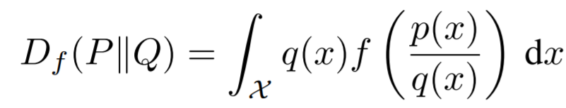
The key thing to keep in mind is that f-divergence aims to to find the difference between two distributions and so the generator function f must be convex, lower-semicontinuous function satisfying f(1) = 0. This is critical for the f-divergence to work correctly. This is specific for the function above and would be different for different functions. f(1) = 0, is important so D_f (P||P) = 0.

Variational Estimation of F-Divergences

Nguyen et al. derived a general variational method to estimate f-divergences given only samples from P and Q. However, the authors of the paper decided to expand upon that and extend their method from estimating divergences for fixed models to estimating model parameters. Hence, the variational divergence minimization (VDM). The VDM framework was invented to show that GANs fall in this class of framework and is a highly specialized version of tha VDM framework.

The shortened proof is as follows:

Continuing off Nguyen et al’s divergence estimation procedure, every convex lower-semicontinuous function (f) has a convex conjugate function (f^*) that is known as the “Fenchel conjugate”. The function is defined below:

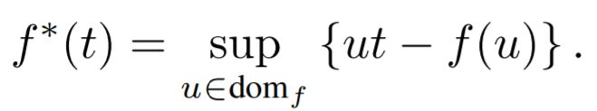
A key characteristic of this function (f*) is that it is also convex and lower-semicontinuous. The creates a duality with f and (f^*) where f** = f. Thus, the function (f) can be rewritten as

As it can be seen in the proof, the importance of the structure of the generator goes beyond the first derivative and is needed for the rest of the calculations to occur. The suprema equation gets used below in the next section of the shortened derivation. Which is as follows:

Continuing from the previous equation and taking from Nguyen et al. a new equation can be created. The equation defined above is a variational representation of f and can be substituted into the definition of f-divergence from Nguyen et al. Doing so will create a lower bound on the divergence as follows:

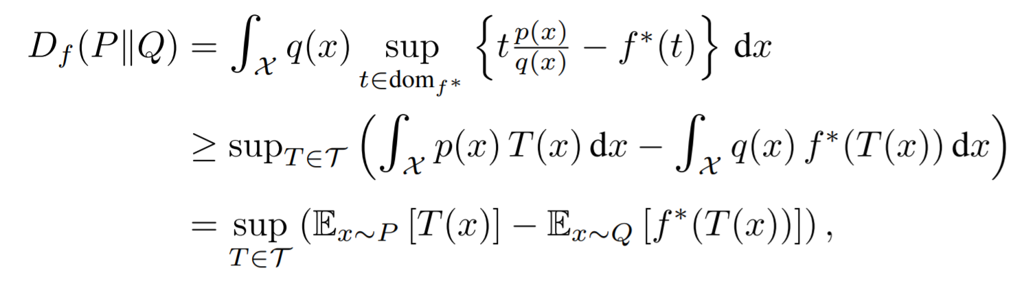
In the equation above there are two types of Ts referenced and so for the sake of this blog post T shall indicate the function T(x) and T~ shall indicate the class that T is contained within.

The T~ is introduced as an arbitrary class of functions but is primarily used to determine which f is the best suited for the situation. The derivation results in a lower bound because of Jensen’s inequality when swapping the integral for a suprema. Another contributing component is that T~ contains only a subset of all possible functions, thus there are only a certain number of possible functions to choose from that fit the requirements.

Thus, we can determine the T that is the best fit taking the variation of the lower bound from the above T and find that the bound is tight for:

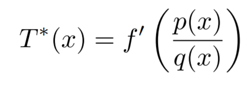
Defining T* is critical as it is the main component in discovering the optimal function (f) for our divergence. The conditional statement helps in choosing f and designing the class of functions T~. Since every divergence will have it’s own unique T* function we need the condition above to construct a consistent function that can accurately portray f.

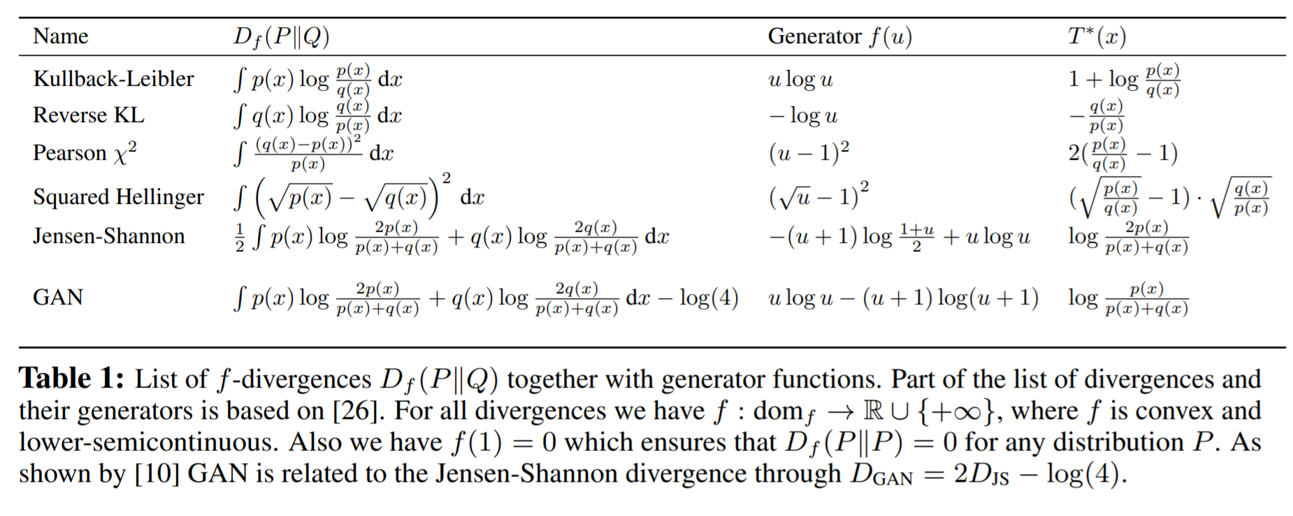
The generated table of relevant divergences and their functions is listed in this table and provides an example of how all these functions differ and their implementation could make profound changes on the applied scenario.

Variational Divergence Minimization (VDM)

All the previous work and definitions were made to fully explain the VDM. The variational lower bound (T) served to figure out the P and Q for D_f(P||Q). P is the true distribution and Q is the generative model that is estimated based off P.

To accomplish this goal the GAN approach is considered. By making use of two neural networks Q and T where Q is the generative model and T is the variational function. Q takes in a random input vector and outputs a sample. T takes in an input and returns a scalar. Q uses the variable θ and T uses w. In terms of creating a parametric equation you get:

The generative model (Q) can be learned by finding a saddle point for the following f-GAN objective where the goal is to minimize θ and maximize w.

The terms in the equation above can be calculated through the following: E_x∼P [·] can be approximated by sampling from the training set without replacement; E_x∼Qθ [·] can be approximated through sampling from the current model. It is important to note to sample the same number from each location.

Running Single-Step Gradient we are able to find a saddle point where Theta is strongly convex and W is strongly concave. There can be many satisfying saddle points and so it comes down to setting a custom metric as to what you want to accept.

VDM vs GAN Construction

The GAN model and VDM model look similar and operate similarly too with how they aim to find a saddle point for maximizing and minimizing certain sections. However, there are some key distinctions between the two.

FGAN:

GAN:

The equations are very similar in appearance but there are some minor discrepancies. The key differences that the D function for GANs is a discriminant function that is more complex than the T lower bound designator function. Also in terms of training speed, maximizing the second term in the F-Gan model is easier than minimizing the second term in the GAN model.

With this you get to see the improvements made and how the VDM expands the capability of a GAN and improves not only its performance in terms of time to compute, but also widens the number of applications that the GAN is able to be used in.

Experiments & Empirical Results

The paper is interesting since it begins talking about f-divergence and expanding on the purpose of f-divergence and their applications. However, the paper ends up with a new model that makes use of f-divergence and variational divergence estimators to make the VDM. This section will consider the success of the VDM. The VDM differs from the traditional GAN and as such is tested differently. The VDM model mainly depends on the divergences that make up the VDM and as such are necessary to test all the various divergences as opposed to just testing the model itself.

Different f-divergences

When testing for different functions to see how well they perform, the researchers came up with this experiment:

Have models learn a Gaussian distribution and find the most optimal parameters to describe the Gaussian distribution. When Q, our model, is turned into a linear function that receives: z ~ N(0,1). Q outputs: G_θ(z) = µ + σz where θ = (µ, σ).

The results of the experiment led to the following table:

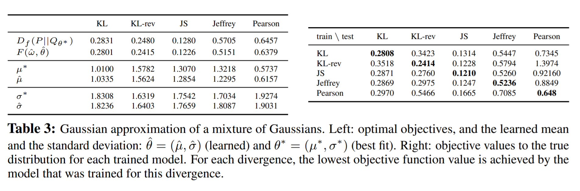
The results of the table affirm the qualities of the VDM. The left side of the table discusses the VDM’s ability to determine the model parameters. This is seen with the µ and σ variables that are meant to show how well the model was able to predict the characteristics as opposed to the best fit / the actual parameters. The right side is a bit less intuitive, but it shows that the models were best fit for the divergence they were trained for. The interesting thing is the dynamic between divergences and well they score when crossfitted with other divergences. This is useful to determine what combinations of divergences are viable options together like for instance using JS and KL for the GAN objective function.

MNIST Digits

Two components to the VDM: Generative Model and Variational Function similar to the GAN. This experiment essentially compares how well the VDM is able to generate MNIST digits using different divergences. The results are compared to a control group. The design of the models that were used for generating were very simple. They made use of a very simple generative model with batch normalization, ReLU, and sigmoid activation functions. The variational function is also simple with a few linear layers and exponential in between.
The VDM is trained as described by sampling without replacement from batches of size 4096. The model is then trained on that information for one hour. The model was compared against variational autoencoders with at least 20 latent dimensions. The results were compiled by doing kernal density estimation and the average log-likelihood was measured for performance.

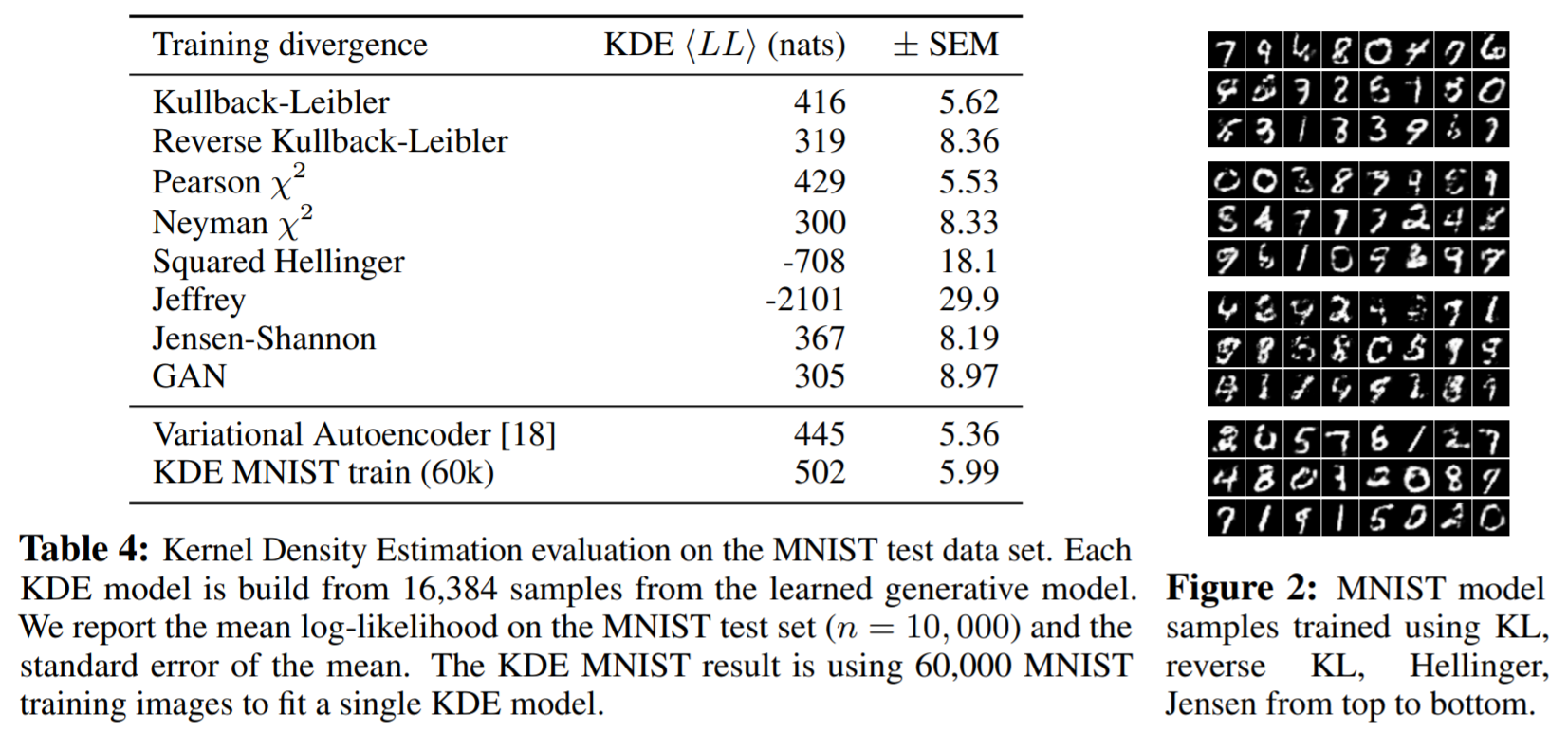
The table and the created outputs for some divergences are displayed. The results for each divergence is given and some basic conclusions can be made. Overall, the performance is all over the place in comparison to the control group, with some divergences performing better than others. The point of the experiment still stands and shows that different divergences and combinations of divergences are better for certain implementations and it comes down to the researchers to figure that out.

Conclusions & Summary

The focus of the paper was more on the GAN feed forward network and how that generative neural sampler could be applied to all generative models. The paper expanded on the concept of f-divergence borrowing from Nguyen et al and drew elements from the traditional GAN to make a new type of GAN, hence the name of the paper f-GAN. Utilizing the proper divergence function leads to the optimal model and better performance and this point was further emphasized with the experiments. The paper contributed the VDM model and the general idea behind the usage of f-Divergence with an application towards GNS / GANs. Thus, GANs can be generalized to an arbitrary divergence function and the algorithm behind GANs is simplified as well.

References

2016 (NeurIPS): S. Nowozin, B. Cseke, R. Tomioka. f-gan: Training generative neural samplers using variational divergence minimization. NeurIPS, 2016.