GAN3 TOWARDS PRINCIPLED METHODS FOR TRAINING GENERATIVE ADVERSARIAL NETWORKS

Introduction

Background

Generative Adversarial Networks (GANs) have achieved great success at generating realistic and sharp looking images. However, they still remain remarkably diffcult to train and most papers at that time dedicated to heuristically finding stable architecture. And there is little to no theory explaining the unstable behaviour of GAN training.

GAN Formulation

GAN in its original formulation, plays the following game:
$\min_G\max_D V(D,G) = \mathbb E_{x\sim p_{data}(x)}[\log D(x)]+\mathbb E_{z\sim p_z(z)}[\log(1-D(G(z)))]$
It can be reformulated as:
$C(G) =\max_D V(G,D)$
$ = \mathbb E_{x\sim p_{data}}[\log D^G(x)]+\mathbb E{z\sim p_z}[\log(1-D^G(G(z)))]$
$ = \mathbb E{x\sim p_{data}}[\log D^G(x)]+\mathbb E{x\sim p_g}[\log(1-D^G(x))]$
$ = \mathbb E{x\sim p_{data}}[\log \frac{p_{data}(x)}{p_{data}(x)+p_g(x)}]+\mathbb E_{x\sim p_g}[\log \frac{p_g(x)}{p_{data}(x)+p_g(x)}]$
and this is called the virtual training criterion.

It can be shown that C(G) is equivalent to the following:
$-\log(4)+2\cdot JSD(p_{data}||p_g)$
where JSD is the Jensen-Shannon divergence:
$JSD(\mathbb P_r||\mathbb P_g)=\frac{1}{2}KL(\mathbb P_r||\mathbb P_A)+\frac{1}{2}KL(\mathbb P_g||\mathbb P_A)$
where $\mathbb P_A$ is the ‘average’ distribution, with density $\frac{P_r+P_g}{2}$.

To train a GAN, we first train the discriminator to optimal, which is maximizing:
$L(D,g_\theta) = \mathbb E_{x\sim \mathbb P_r}[\log D(x)]+\mathbb E_{x\sim \mathbb P_g}[\log(1-D(x))]$
and the optimal discriminator is obatined as:
$D^*(x) = \frac{P_r(x)}{P_r(x)+P_g(x)}$

Plug in the optimal discriminator to $L(D,g_\theta)$, we get:
$L(D^*, g_\theta) = 2JSD(\mathbb P_r||\mathbb P_g)-2\log2$
So, minimizing $L(D,g_\theta)$ as a function of $\theta$ gives the minimized Jensen-Shannon divergence when the discriminator is optimal.

In theory, we would first train discriminator as close to optimal as we can, then do gradient steps on $\theta$, and alternating these two things to get our generator. \color{red} But this doesn’t work. In practice, as the discriminator gets better, the updates to the generator get consistently worse

Main Contribution

Based on the problem regarding GAN training, the authors proposed 4 questions to be answered:

1. Why do updates get worse as the discriminator gets better? Both in the original and the new cost function.
2. Why is GAN training massively unstable?
3. Is the new cost function following a similar divergence to the JSD? If so, what are its properties?
4. Is there a way to avoid some of these issues?

We first take a look at the source of instabilities

Sources of Instability

Discontinuity Conjecture

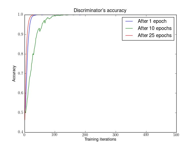
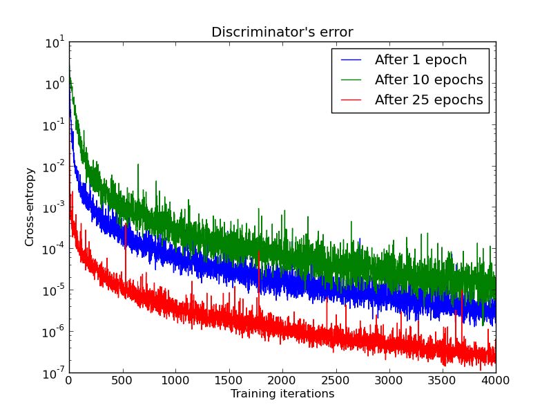
From the cost function and the optimal discriminator, we ‘know’ that the trained discriminator will have cost of at most $2\log2-2JSD(\mathbb P_r||\mathbb P_g)$. However, in practice, if we train D till convergence, its error will go to 0, pointing to the fact that the JSD between them is maxed out. The only way this can happen is if the distributions are not continuous, or they have disjoint supports. And one possible cause for the distribution to be discontinuous is if their supports lie on low dimensional manifolds. Previous work on GAN showed strong empirical and theoretical evidence to believe that $\mathbb P_r$ is indeed extremely concentrated on a low dimensional manifold. And the authors proved that this is the case as well for $\mathbb P_g$.

Below regards DCGAN trained for 1,10,25 epochs. Then, with generator fixed, train a discriminator from scratch.

Lemma 1

Let $g:\mathcal Z\rightarrow\mathcal X$ be a function composed by affine transformations and pointwise non-linearities, which can either be rectifiers, leaky rectifiers, or smooth strictly increasing functions (such as the sigmoid, tanh, softplus, etc). Then, $g(\mathcal Z)$ is composed in a countable union of manifolds of dimension at most dim $\mathcal Z$. Therefore, if the dimension of $\mathcal Z$ is less than the one of $\mathcal X$, $g(\mathcal Z)$ will be a set of measure 0 in $\mathcal X$.

The intuition behind this lemma is $\mathbb P_g$ is defined via sampling from a simple prior $z\sim p(z)$, and then applying a function $g:\mathcal Z\rightarrow\mathcal X$, so the support of $\mathbb P_g$ has to be contained in $g(\mathcal Z)$. If the dimensionality of $\mathcal Z$ is less than the dimension of $\mathcal X$, then it’s impossible for $\mathbb P_g$ to be continuous.

Perfect Discrimination Theorem

Theorem 2.1

If two distributions $\mathbb P_r$ and $\mathbb P_g$ have support contained on two disjoint compact subsets $\mathcal M$ and $\mathcal P$ respectively, then there is a smooth optimal discriminator $D^*:\mathcal X\rightarrow [0,1]$ that has accuracy 1 and $\nabla_xD^*(x)=0 \forall x\in \mathcal M\cup\mathcal P$.

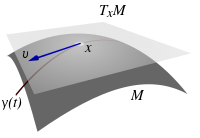
Definition (Transversal Intersection)

Let $\mathcal M$ and $\mathcal P$ be two boundary free regular submanifolds of $\mathcal F$, which in our case will simply be $\mathcal F = \mathbb R^d$. Let $x\in \mathcal M\cap \mathcal P$ be an intersection point of the two manifolds. We say that $\mathcal M$ and $\mathcal P$ intersect transversally in $x$ if $\mathcal T_x\mathcal M+\mathcal T_x\mathcal P = \mathcal T_x\mathcal F$, where $\mathcal T_x\mathcal M$ means the tangent space of $\mathcal M$ around $x$.

Definition (Perfect Alignment)

We say that two manifolds without boundary $\mathcal M$ and $\mathcal P$ \textbf{perfectly align} if there exists $x\in \mathcal M \cap \mathcal P$ such that $\mathcal M$ and $\mathcal P$ don’t intersect transversally in $x$. And let $\partial\mathcal M$ and $\partial\mathcal P$ denote the boundary of manifolds $\mathcal M$ and $\mathcal P$, we say $\mathcal M$ and $\mathcal P$ are perfectly align if any of the boundary free manifold pairs ($\mathcal M$, $\mathcal P$), ($\mathcal M$, $\partial\mathcal P$), ($\partial\mathcal M$, $\mathcal P$),($\partial\mathcal M$, $\partial\mathcal P$) perfectly align.

Lemma 2

Let $\mathcal M$ and $\mathcal P$ be two regular submanifolds of $\mathbb R^d$ that don’t have full dimension. Let $\eta, \eta'$ be arbitrary independent continuous random variables. We therefore define the perturbed manifolds as $\mathcal{\tilde M}=\mathcal M+\eta$ and $\tilde{\mathcal P}=\mathcal{P}+\eta'$. Then [\mathbb P_{\eta, \eta’}(\mathcal{\tilde M} \text{ does not perfect align with }\mathcal{\tilde P}) = 1]

This implies that, in practice, we can safely assume that any two manifolds never perfectly assign, since arbitrarilly small perturbation on two manifolds will lead them to intersect transversally or don’t intersect at all.

Lemma 3

Let $\mathcal M$ and $\mathcal P$ be two regular submanifolds of $\mathbb R^d$ that don’t perfectly align and don’t have full dimension. Let $\mathcal L=\mathcal M\cap\mathcal P$. If $\mathcal M$ and $\mathcal P$ don’t have boundary, then $\mathcal L$ is also a manifold, and has strictly lower dimension than both the one of $\mathcal M$ and the one of $\mathcal P$. If they have boundary, $\mathcal L$ is a union of at most 4 strictly lower dimensional manifolds. In both cases, $\mathcal L$ has measure 0 in both $\mathcal M$ and $\mathcal P$.

If two manifolds don’t perfectly align, their intersection $\mathcal L=\mathcal M\cap\mathcal P$ will be a finite union of manifolds with dimensions strictly lower than both the dimension of $\mathcal M$ and $\mathcal P$.

Theorem 2.2 (The Perfect Discrimination Theorem)

Let $\mathbb P_r$ and $\mathbb P_g$ be two distributions that have support contained in two closed manifolds $\mathcal M$ and $\mathcal P$ that don’t perfectly align and don’t have full dimension. We further assume that $\mathbb P_r$ and $\mathbb P_g$ are continuous in their respective manifolds, meaning that if there is a set A with measure 0 in $\mathcal M$, then $\mathbb P_r(A)=0$ (and analogously for $\mathbb P_g$). \color{red} Then, there exists an optimal discriminator $D^*:\mathcal X\rightarrow[0,1]$ that has accuracy 1 and for almost any x in $\mathcal M$ or $\mathcal P$, $D^*$ is smooth in a neighbourhood of $x$ and $\nabla_xD^*(x)=0$.

Combining the two theorems (2.1 and 2.2) stated together tells us that there are perfect discriminators which are smooth and constant almost everywhere in $\mathcal M$ and $\mathcal P$. And the fact that the discriminator is constant in both manifolds points to the fact that we won’t be able to learn anything by backproping through it.

Theorem 2.3

Let $\mathbb P_r$ and $\mathbb P_g$ be two distributions whose support lies in two manifolds $\mathcal M$ and $\mathcal P$ that don’t have full dimension and don’t perfectly align.
We further assume that $\mathbb P_r$ and $\mathbb P_g$ are continuous in their respective manifolds. Then,
$JSD(\mathbb P_r||\mathbb P_g)=\log2$
$KL(\mathbb P_r||\mathbb P_g)=+\infty$
$KL(\mathbb P_g||\mathbb P_r)=+\infty$

This implies:

1. divergences will be maxed out even if the two manifolds lie arbitrarilly close to each other (impossible to apply gradient descent)
2. samples of our generator might look impressively good, yet both KL divergences will be infinity
3. attempting to use divergences out of the box to test similarities between the distributions we typically consider might be a terrible idea

Vanishing Gradients on the Generator

Denote $||D||=\sup_{x\in\mathcal X}|D(x)|+||\nabla_xD(x)||_2$
(Note: The authors stated that this norm is used to make proofs simpler, and can be replaced with Sobolev norm $||\cdot||_{1,p}$ for $p<\infty$ covered by the universal approximation theorem in the sense that we can guarantee a neural network approximation in this norm)

Theorem 2.4

Let $g_\theta:\mathcal Z\rightarrow\mathcal X$ be a differentiable function that induces a distribution $\mathbb P_g$. Let $\mathbb P_r$ be the real data distribution. Let D be a differentiable discriminator. If the conditions of Theorem 2.1 and 2.2 are satisfied, $||D-D^*||<\epsilon$, and $\mathbb E_{z\sim p(z)}[||J_\theta g_\theta(z)||^2_2]\le M^2$, then
$||\nabla_\theta\mathbb E_{z\sim p(z)}[\log(1-D(g_\theta(z)))]||_2<M\frac{\epsilon}{1-\epsilon}$

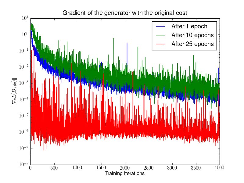
Theorem 2.4 shows that as our discriminator gets better, the gradient of the generator vanishes.
And the figure below shows an experimental verfication of the above statement. First train a DCGAN for 1, 10 and 25 epochs. Then, with the generator fixed train a discriminator from scratch and measure gradients with the original cost function.

The $-\log D$ Alternative

In original GAN paper, the authors conjectured that the instable behaviour is because of the choose of loss function so they proposed an alternative to “fix” it, but even with the alternative loss function, the problem remains, and yet little is known about the nature of the alternative loss.

To avoid vanishing gradient when the discrminator is very confident, an alternative gradient step for the generator is used:
$\Delta\theta=\nabla_\theta\mathbb E_{z\sim p(z)}[-\log D(g_\theta(z))]$

Theorem 2.5

Let $\mathbb P_r$ and $\mathbb P_{g_\theta}$ be two continuous distributions, with densities $P_r,P_{g_\theta}$ respectively. Let $D^*(x) = \frac{P_r(x)}{P_r(x)+P_{g_\theta}(x)}$ be the optimal discriminator, fixed for a value $\theta_0$. Therefore,
$\mathbb E_{z\sim p(z)}[-\nabla_\theta\log D^*(g_\theta(z))|_{\theta=\theta_0}] =\nabla_\theta[KL(\mathbb P_{g_\theta}||\mathbb P_r)-2JSD(\mathbb P_{g_\theta}||\mathbb P_r)]|_{\theta=\theta_0}$

Theorem 2.6

Let $g_\theta:\mathcal Z\rightarrow \mathcal X$ be a differentiable function that induces a distribution $\mathbb P_g$. Let $\mathbb P_r$ be the real data distribution, with either conditions of Theorems 2.1 and 2.2 satisfied. Let D be a discriminator such that $D^*-D=\epsilon$ is a centered Gaussian process indexed by $x$ and independent for every $x$ and $\nabla_xD^*-\nabla_xD=r$ another independent centered Gaussian process indexed by $x$ and independent of every $x$. Then, each coordinate of
$\mathbb E_{z\sim p(z)}[-\nabla_\theta\log D(g_\theta(z))]$
is centered Cauchy distribution with infinite expectation and variance.

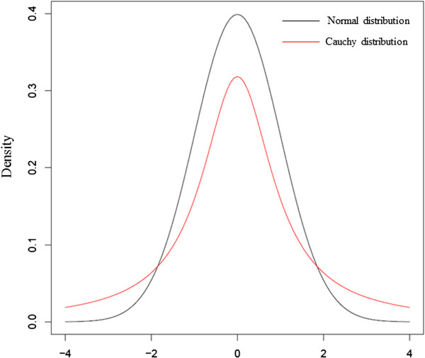
Theorem 2.6 implies that we would have large variance in gradients, and the instable update would actually lower sample quality. Moreover, the fact that the distribution updates are centered means that, if we bound the updates, the expected update would be 0, providing no feedback to the gradient.

Towards Softer Metrics and Distributions

Break Assumptions

To fix the Instability and vanishing gradients issue, we need to break the assumptions of previous theorems. And the authors choose to add continuous noise to the inputs of the discriminator, therefore, smoothening the distribution of the probability mass.

Theorem 3.1

If X has distribution $\mathbb {P_X}$ with support on $\mathcal M$ and $\epsilon$ is an absolutely continuous random variable with density $P_\epsilon$, then $\mathbb P_{X+\epsilon}$ is absolutely continuous with density
$P_{X+\epsilon}=\mathbb E_{y\sim\mathbb P_X}[P_\epsilon(x-y)]$
$ = \int_{\mathcal M}P_\epsilon(x-y)d\mathbb P_X(y)$

Theorem 3.2

Let $\mathbb P_r$ and $\mathbb P_g$ be two distributions with support on $\mathcal M$ and $\mathcal P$ respectively, with $\epsilon\sim\mathcal N(0,\sigma^2I)$. Then, the gradient passed to the generator has the form
$\mathbb E_{z\sim p(z)}[\nabla_\theta\log(1-D^*(g_\theta(z)))]$
$= \mathbb E_{z\sim p(z)}[a(z)\int_{\mathcal M}P_\epsilon(g_\theta(z)-y)\nabla_\theta||g_\theta(z)-y||^2d\mathbb P_r(y)$
$-b(z)\int_{\mathcal P}P_\epsilon(g_\theta(z)-y)\nabla_\theta||g_\theta(z)-y||^2d\mathbb P_g(y)]$
This theorem proves that we will drive our samples $g_\theta(z)$ towards points along the data manifold, weighted by their probability and the distance from our samples.

To protect the discriminator from measure 0 adversarial examples, it is important to backprop through noisy samples in the generator as well.

Corollary

Let $\epsilon,epsilon'\sim\mathcal N(0,\sigma^2I)$ and $\tilde g_\theta(z) = g_\theta(z) + \epsilon'$, then
$\mathbb E_{z\sim p(z)}[\nabla_\theta\log(1-D^*(\tilde g_\theta(z)))]$
$ = \mathbb E_{z\sim p(z)}[a(z)\int_{\mathcal M}P_\epsilon(\tilde g_\theta(z)-y)\nabla_\theta||\tilde g_\theta(z)-y||^2d\mathbb P_r(y)-b(z)\int_{\mathcal P}P_\epsilon(\tilde g_\theta(z)-y)\nabla_\theta||\tilde g_\theta(z)-y||^2d\mathbb P_g(y)]$
$= 2\nabla_\theta JSD(\mathbb P_{r+\epsilon}||\mathbb P_{g+\epsilon})$

Wasserstein Metric

The other way to go is to use Wasserstein Metric to replace traditional JSD distance.

Definition

[W(P,Q)=\inf_{\gamma\in\Gamma}\int_{\mathcal X\times\mathcal X}||x-y||_2d\gamma(x,y)] where $\Gamma$ is the set of all possible joints on $\mathcal X\times\mathcal X$ that have marginals P and Q.

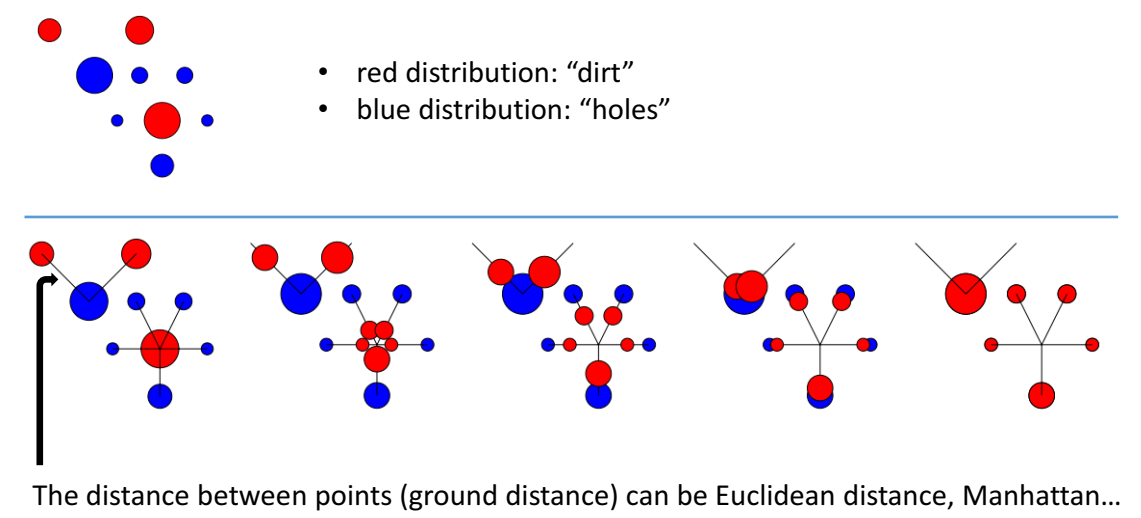
Wasserstein Distance is also called Earth Mover’s Distance (EMD), it’s the minimum cost of transporting the whole probability mass of P from its support to match the probability mass of Q on Q’s support.

Intuitively, given two distributions, one can be seen as a mass of earth properly spread in space, the other as a collection of holes in that same space. Then, the EMD measures the least amount of work needed to fill the holes with earth. Here, a unit of work corresponds to transporting a unit of earth by a unit of ground distance.

Lemma 4

Let $\epsilon$ be a random vector with mean 0, then we have
$W(\mathbb P_X,\mathbb P_{X+\epsilon})\le V^{\frac{1}{2}}$
where $V=\mathbb E[||\epsilon||^2_2]$ is the variance of $\epsilon$.

Theorem 3.3

Let $\mathbb P_r$ and $\mathbb P_g$ be any two distributions, and $\epsilon$ be a random vector with mean 0 and variance V. If $\mathbb P_{r+\epsilon}$ and $\mathbb P_{g+\epsilon}$ have support contained on a ball of diameter C, then
$W(\mathbb P_r,\mathbb P_g)\le 2V^{\frac{1}{2}}+2C\sqrt{JSD(\mathbb P_{r+\epsilon}||\mathbb P_{g+\epsilon})}$

This theorem implies that Wasserstein Distance can be controlled since both parts of this upper bound can be manually controlled.