GAN5 Generalization and Equilibrium in Generative Adversarial Nets (GANs)

Intro

This blog post focuses on the paper Generalization and Equilibrium in Generative Adversarial Nets (GANs) and focuses on the concept of generalization with applications to GANs. The paper introduces the concept of generalization and the fact that the GAN model does not perform good generalization. The paper introduces a new type of distance measure to better calculate the generalization factor. The paper subsequently comes up within a new model called the MIX-GAN which focuses on demonstrating the importance of generalization when it comes to GAN training. The paper aims to help reader’s understand the purpose of the GAN model and how the model can be improved through the implementation of generalization while training the GAN.

​

​

Background

GANs were first introduced by Goodfellow et al. 2014 and the Goodfellow GAN can be described as follows:
GANs are type of generative model used to come up with images or other samples to imitate real life samples. In more detail, the objective of the GAN when it comes to training a generator deep net whose input is a standard Gaussian, and whose output is a sample from some real distribution.

GANs work by comparing two distributions, as mentioned above, where the generator net part of the GAN attempts to “fool” the discriminator function into thinking that the generated image is a real image. This dual system is trained through backpropagation of the result from the discriminator that feeds into the generator. Thus the relationship between the generator and the discriminator can be thought of as a game between two players solving a min max scenario. This concept is further explored within the paper. The min max game is critical to understanding GANs and how they are trained.

(traditional GAN training objective from Goodfellow 2014)

​
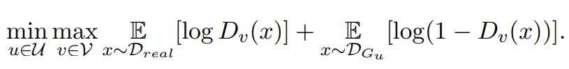
In more detail the GAN objective function aims to minimize the output from the generator but the opposite is true for the discriminator which aims to maximize the result. The result is the label assigned to the training sample and then re-evaluated in the long term.
​

Generalization

The definition of generalization in terms of GANs is related to how well the GAN is able to imitate the real distribution. A lot of the times the discriminator will be fooled but the derived distribution from the GAN model is weak and very ill representative of the actual distribution. Standard metrics are not as useful as measuring whether the distribution is close or not. Often there are times the GAN is able to train successfully to imitate the real distribution but according to standard metrics the trained distribution is deemed extremely different than the actual distribution, even though it might not be. Generalization is important when it comes to describing when the generator has won. At this point you need to consider is the created distribution and the real distribution the same or at least similar? This is tough to do when you have complicated distributions that have many valleys and peaks. Take for example this distribution:

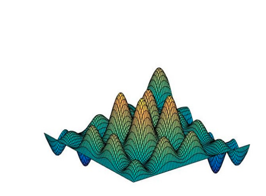
The distribution as mentioned has many peaks and valleys and when considering this distribution with high dimensionality there could be an exponential number of extrema. Sampling becomes a big issue. How do you sample so that all the extrema are accurately represented? How large would the sample size need to be for this to work? These questions are the underlying issue when it comes to modeling and working high dimensionality and complex distributions. The simple answer boils down to having a sample size of exponential size as well. However, that isn’t feasible and thus needs to be made more realistic.

Generalization Math

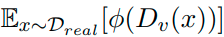
Let x1…xm be the training examples and let D^{^}_real be the uniform distribution for x₁…x_m. Also let G_u(h1)…G_u(hr) be a set of r examples from the generated distribution D_G. In training, we use:

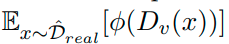
to approximate the value of:

Attempt to minimize the distance (or divergence) between D^{^}_real and D_G. This can be done to a certain extreme and so the final simplified version of this equation can be represented as:

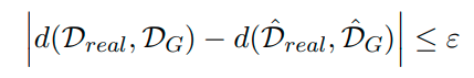
The equation above gives a more concrete mathematical equation for Generalization and it can explained as the following: “generalization in GANs means that the population distance between the true and generated distribution is close to the empirical distance between the empirical distributions. Our target is to make the former distance small, whereas the latter one is what we can access and minimize in practice. The definition allows only polynomial number of samples from the generated distribution because the training algorithm should run in polynomial time.” The concept is a little confusing but can be simplified to this: in an ideal world we can draw an infinite number of samples from the true distribution to get the value for D_real, however; in practicality that is not possible and so we have the empirical distance with a finite number of samples to estimate the expected value of the real distribution as seen above. The equation above takes it a step further and explicates that the distance between the empirical true distribution and empirical generated distribution is as close as it can be to the population distance between the population true distribution and the population generated distribution. The population distance is calculated theoretically and used in the calculation. Thus, the calculation is completed with an error bound that acts as measurement for the difference between the two distances. If the empirical distance is close enough to the population distance within this error bound, we can consider the empirical distance to be the same as the population distance.

Neural Net Distance

The paper brings up a problem with current metrics and that they are a bad method of measuring how well the generated distribution follows and imitates the original distribution. So, the authors behind the paper came up with a new measuring metrics strictly to see how well two distributions match each other. This metric is the neural net distance metric.

Neural Net Distance is derived from the f-divergence concept and follows the derivation of the f-divergence function closely.

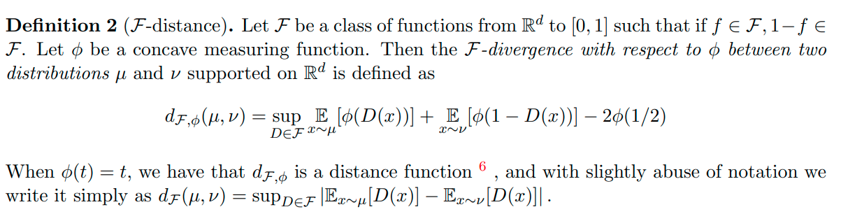
For example when φ(t) is log(t) and F = {all functions from R^d mapped to [0, 1]} then the derived equation above is equal to JS divergence. However, when φ(t) is t and F = {all 1-Lipschitz functions from R^d mapped to [0, 1]} then the equation above is equal to Wasserstein distance.

• (Lipschitz functions are mentioned and Lipschitz refers to the training parameters and indicates that changing a parameter by delta changes the output of the deep net by less than constant * delta.)

All this is to indicate that the distance metric is variable and changes with what kind of base GAN you are working with / what kind of distribution you’d like to measure.

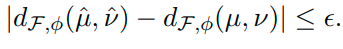
GAN training uses F to be a class of neural nets with a bound p on the number of parameters. An assumption can be made regarding the measuring function such that it takes in values between [−∆, ∆] and that it is L_φ-Lipschitz.

Even more so, F is a class of discriminators that is L-Lipschitz to the target distribution where p denotes the number of parameters in the target distribution.

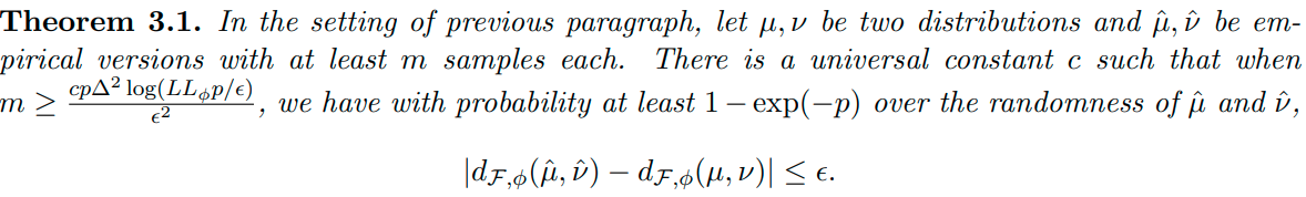
In a general sense you get the equation:

The downside of the Neural Net Distance is that it will return a small value even if u and v are are far from each other. This is due to the capacity being limited by p.

Equilibrium & Mixtures

The idea of equilibrium stems from the GAN min max problem. When trying to train and optimize a GAN the generator must be minimized and the discriminator needs to be maximized. Equilibrium seeks a state where both the discriminator and the generator cannot be optimized further. The thing to keep in mind is that the saddle point reached is not necessarily zero. This paper puts a spin on that and recognizes an “equilibrium” value where generator is always less than or equal to this value. Conversely, the discriminator is always greater or equal to this value as demonstrated below.

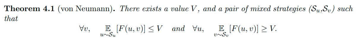
The S value seen in the theorem is used to represent the strategies that the discriminator and generator use respectively. The strategies are unchanged and so there is no changing of strategies once the other player’s strategy is revealed. Each player still performs to the best of their ability keeping in mind their initial strategy.

The paper focuses only on the generator side as opposed to the disciminator. The reasons for the focus on the generator only is as follows:

• Payoff is generated by the generator:
  
  The payoff is generated by the generator first sample u ∼ S_u, h ∼ D_h. This results in an example that is generated x = G_u(h).

• Mixed Generator Composition vs. Mixed Discriminator:
  
  The mixed generator is compromised of a linear mixture of generators. The mixed discriminator is more complicated since the objective function of the discriminator may not be linear. Thus, when accounting for the objective function it escapes a linear space; otherwise the mixed discriminator would also be linear.

• Output of Discriminator is not important:
  
  The output of the discriminator mixture is not important for consideration since the mixture is also unable to differentiate between the generated and actual distribution effectively.

All these scenarios are resolved using a mixture generator and approximating the difference between the two distributions to a certain error value (as seen with all the formulas above).

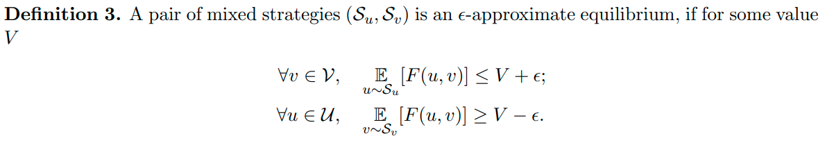
This is what the strategies come out to be after accounting for a small margin of error. The basic idea here is that it takes O§ (where p is the number of parameters in the sample set) to approximate a quality distribution that is able to imitate the real distribution while accounting for the error.

There is a more complex version of this that takes into account pure strategies. The paper does not go into details about pure strategies but discusses a short overview about them. The idea boils down to the concept of mixtures, there is not much change from what is already written in this blog besides the fact that if a pure strategy is attempted then the complexity increases to O(p²) since each network compromises of O§ size and then those are used to make the mixture generator in a linear fashion.

MIX-GAN

A mix GAN is a GAN that makes use of the idea of a mixture of generators within reason. So they make use of a mixture of T components, where T is constrained by GPU memory (< 5). Maintain T generators and T discriminators. All the respective weights for each generator is maintained and everything is trained through backwards propagation. The specific softmax used for training is listed below.

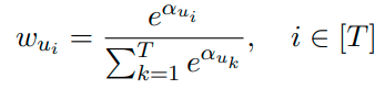
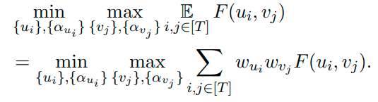
The softmax function is critical for defining the weights which in turn are needed for the payoff function for the MIX+GAN. You can think of it as the original min max problem for the GAN as the structure of the equations are similar.

Empirical Results

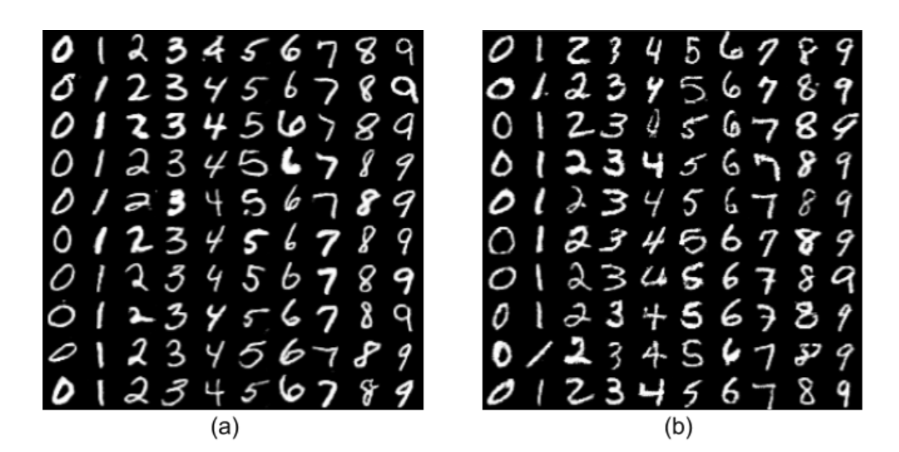
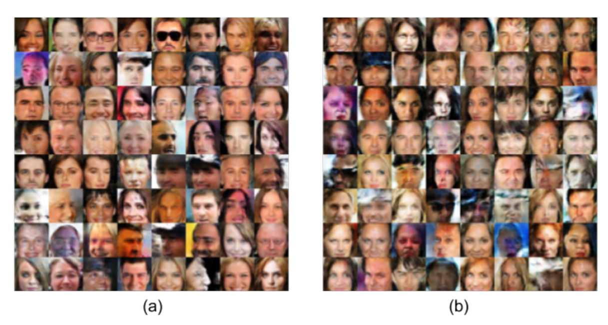
The examples above show the comparison between a typical DC-GAN and a MIX-DCGAN. The MIX-GAN is represented by the A side and the normal DCGAN is represented by the B side. THe interesting thing to note is the quality of the results of the GANs. The MIX-GAN performed slightly better in terms of more clear output compared to the results of the regular GAN.

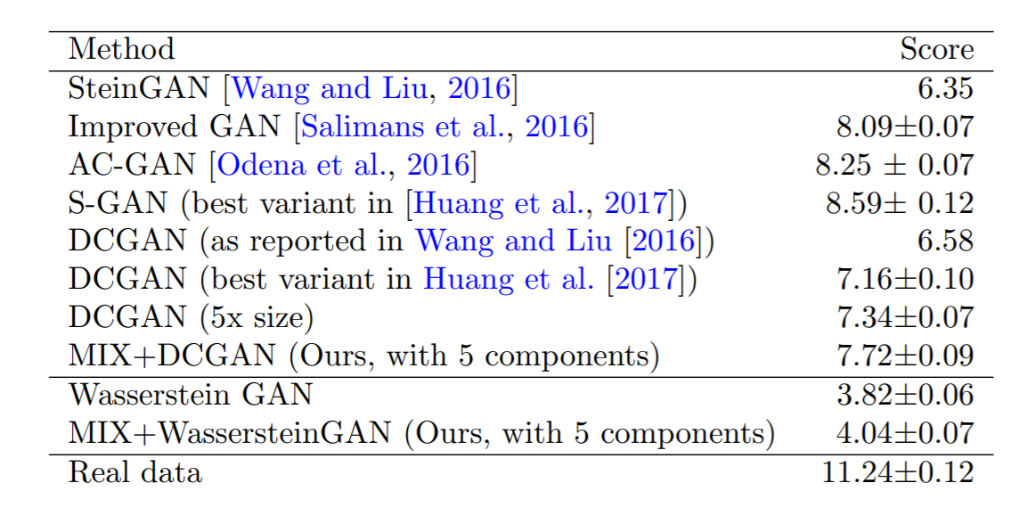
This is further evidenced by the results of the CIFAR-10 test results. The MIX-GAN is able to compete to the same performance level of the GAN that it models. At times it does better than the GAN model that it is imitating. The most curious thing about the MIX-GAN is ability to be small and retain very little parameters yet be able to compete with more complex and larger GANs, as seen with the MIX-DCGAN and DCGAN (5x time) size scores.

Conclusions

The concept of the MIX-GAN leads to more efficient GANs. They are typically smaller and perform the same as the normal version of the particular GAN model that they are attempting to turn into a mixture through the measuring function. The MIX-GAN allows for more quality samples and more diverse samples from the generated distribution because it is able to better reflect the true distribution unlike other GANs. On a theoretical standpoint this paper focused mainly improving the GAN’s ability to come to a good stopping point that properly reflects the true distribution. Many GANs fail to do this hence the team’s research into generalization and the neural net distance metric for a better way to determine if the generated distribution and real distribution are similar or not.

References

2017 (ICML): S. Arora, R. Ge, Y. Liang, T. Ma, Y. Zhang. Generalization and equilibrium in generative adversarial nets (GANs). ICML, 2017.