NODE1 Neural ODE
Anurendra Kumar (ak32@illinois.edu) https://anurendra.github.io/
Abstract
Today we’ll talk about the popular Neural ODE paper which won best paper award in Neurips 2018. This paper develops a foundational framework for infinitely many layered deep neural networks. The framework allows us to take advantage of the extensive research on ODE Solvers.
Background : Ordinary Differential Equations
In physics, Ordinary Differential Equations(ODEs) have been often used to describe the dynamics and referred as a vector field of the underlying physical system.

A system of ODEs can be represented as,
Neural ODEs aims to replace explicit ODEs by an ODE with learnable parameters. In past, extensive research has been done on explicit and implicit ODESolvers which aims to solve an ODE(forward pass). The simplest ODE solver Forward Euler method works by moving along the gradient from a starting point:
Sophisticated higher order explicit ODE solvers like Rungakutta have low error margin.
An example of implicit ODE Solver is Backward Euler Method:
The implicit solvers are computationally expensive but often has better approximation guarantees. Various adaptive-step size solvers have been developed which provide better error handling.
Problem Setup: Supervised learning
Traditional Machine learning solves: , where, is label and is input features. Neural ODEs views the same problem as an ODE with Initial value problem,
where the value at initial time point is input features and the label is the value at final time point. For now, Let’s assume that and have same dimensionality for simplicity. Neural ODE aims to learn an invertible transformation between and .
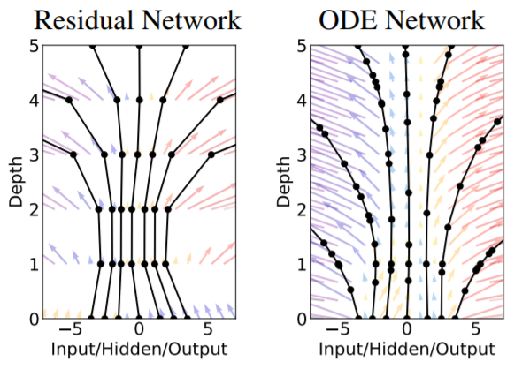
The idea of viewing supervised learning as an ODE system came by observing the updates in Resnet. In Resnet, the updates in -th layer is as follows,
We can view above update as the euler discretization of a continuous dynamic system,
We can therefore view each layer as an euler update in an ODE solver with dynamics .
Infinite layers: ODE Solver as foward pass
Did you ever think that a DNN can have infinite layers? If we try to implement it naively by having different parameters in each layer, then there are two prominent issues we’ll be facing,
i)Overfitting
ii)Memory issues. This is because each layer with learnable parameters in DNN needs to store its input until the backward pass. So, it’s not practically feasible in traditional setting.
A natural question arises that “why can’t we have infinite updates in ODE solver instead of updates?”, where denotes number of euler steps or layers. We just need to use state of the art adaptive ODE Solvers which is memory efficient (more discussed later).
Neural Ordinary Differential equations
Here we summarize the underlying idea of Neural ODE. Instead of trying to solve for , Neural ODE solves, , given the initial condition . The parametrization is done as,
The existing ODE Solvers are used for forward pass.
Backpropagation through Neural ODE
Ultimately we want to optimize some loss w.r.t. parameters ,
If loss is mean squared error, then we can write, . Without loss of generality, we’ll primary focus on computing . If we know the ODE solver, then we can backprop through the solver using automatic differentiation. However, there are two issues with this approach,
i) Backpropagation is dependent on ODE Solvers, this is not desirable. Ideally, we would like to treat ODE Solver as a black box.
ii) If we use “implicit” solvers which often perform inner optimization, then the backpropagation using automatic differentiation is memory intensive.
Adjoint sensitivity analysis: Reverse-mode Autodiff
This paper borrows an age old idea of adjoint based methods from ODE literature to perform backprobagation with respect to parameters in constant memory and without having the knowledge of ODE Solver. To compute we need to compute . Therefore, let’s define the adjoint state . In the case of Resnet, the adjoint state has following updates during backpropagation,
You might have observed that updates of adjoint is an euler step in backward direction with a known dynamics. You guessed it, right. The adjoint state in continuous setting follows following dynamics in backward direction,
For Resnet, the updates of loss is,
Similarly, loss in continuous setting follows a dynamics in the backward direction,
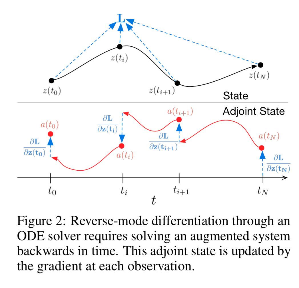
Thus, during the backward pass of , we also need to do a backward pass on and . The vector jacobian products and can be computed using automatic differentiation in similar time cost as of . The full algorithms for all three backward dynamics is shown below,

Results
Experiment 1 : Supervised Learning
The paper performs a supervised learning on MNIST data. It uses resnet and multi-layered perceptron as baselines. The result is shown below,
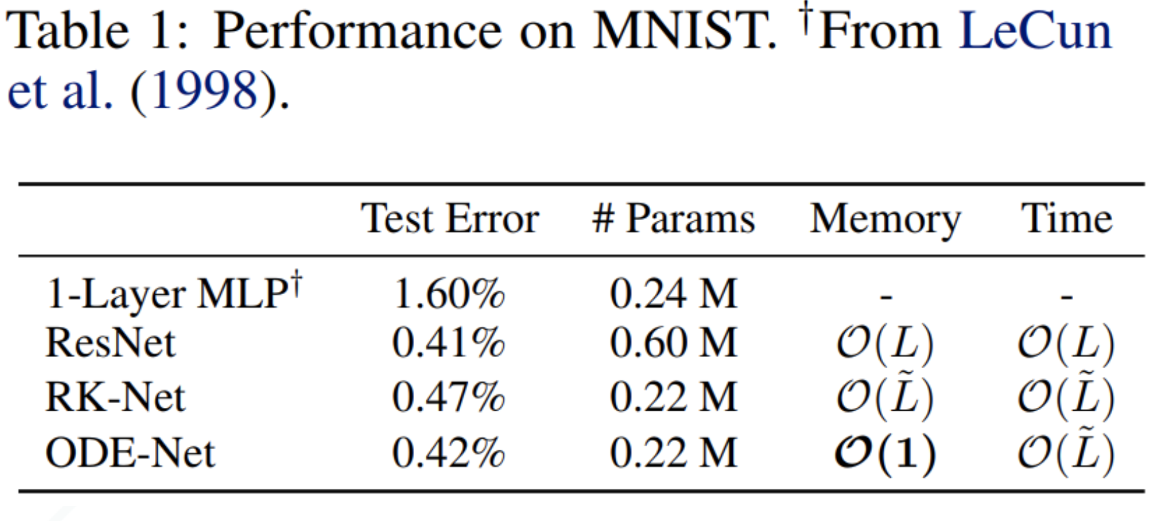
RK-Net uses Runga kutta for forward pass and automatic differentiation for backward pass. We can see that ODENet has fewer parameters with similar accuracy and constant memory.
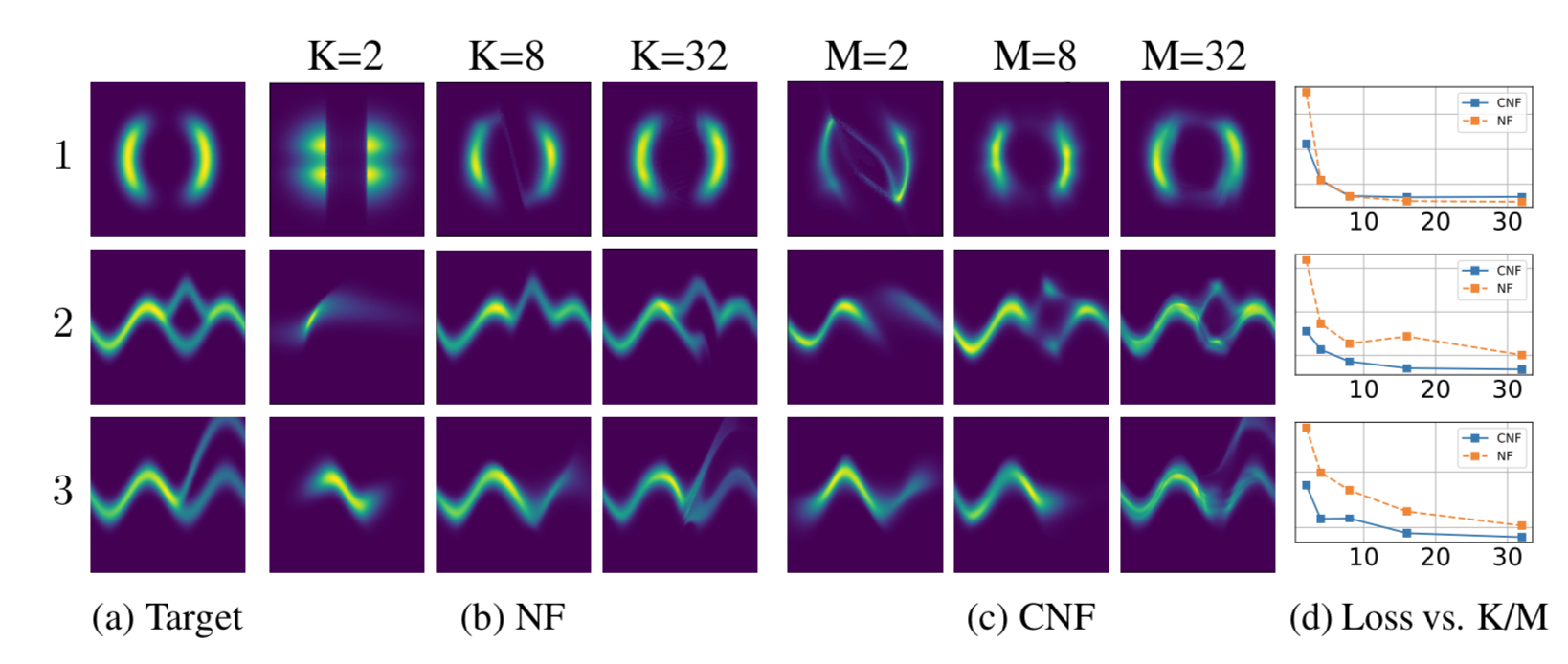
Experiment 2 : Normalizing flows
The paper proposes a continuous version of normalizing flows. Traditionally normalizing flows is enabled using change of variable formula. This paper proposes instantaneous change of variables formula using ODE dynamics.

The results are shown belo,
Time Series Latent ODE
Traditional Rnns can only utilize regular time interval signals in its vanilla form. Neural ODE allows us to sample from a continuous dynamic system,
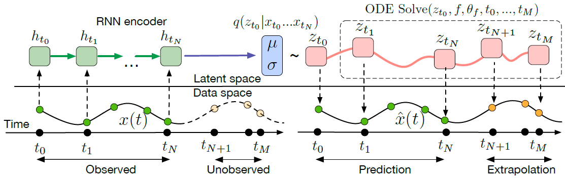
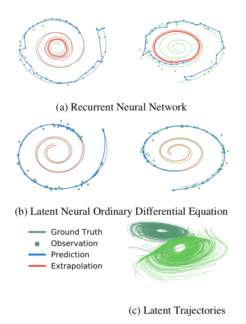
The result for both the RNN and neural ODE for continuous time series for a spiral synthetic data is shown below. It can be seen that RNNs learn very stiff dynamics and have exploding gradients while ODEs are guaranteed to be smooth.
Conclusion
Personally, I believe that this is a phenomonal paper which has enabled us to have infinite layers, handle continuous time series and normalizing flow in constant memory by using the state of the art ODE Solvers. It’s impact on learning dynamics for physical and biophysical system would be immense in future.
References
Chen, R. T., Rubanova, Y., Bettencourt, J., & Duvenaud, D. (2018). Neural ordinary differential equations. arXiv preprint arXiv:1806.07366.