VAE1 Importance Weighted Autoencoders

Importance Weighted Autoencoders: what makes a good ELBO in VAE?

Variational AutoEncoders (VAE) [1] is a powerful generative model which combines the variational inference and autoencoders together. It approximates the posterior distribution with a simple and tractable one, and optimize the lower bound of the true data distribution, which is called evidence lower bound (ELBO). Althoug optimizing ELBO is effective in practice, this estimation is actually biased, and it’s shown that this bias actually cannot be eliminated in vanilla VAE. Here we introduce a work that tries to minimize this bias called Importance Weighted Autoencoders (IWAE) [2], along with its variants which combines the objective in VAE and IWAE.

Introduction to VAE and ELBO

VAE consists of the encoder $q_{\phi}$ and the decoder $p_{\theta}$. It first encodes each sample $x$ into a distribution of the latent variables $q_{\phi}(\cdot|x)$. Then the latent variables are sampled from the distibution as $z\sim q_{\phi}(z|x)$. The latent variables serve as the input to the decoder where the reconstructed output is $\hat{x}\sim p_{\theta}(x|z)$. The overview of VAE is shown in Fig 1.

Fig 1. Overview of VAE (source from [1])

The training objective of VAE is to maximize ELBO. There are multiple ways to derivate ELBO, and one way is through the Bayesian theory. $\log{p_{\theta}(x)}$ can be rewritten as

$$\begin{align} \log{p_{\theta}(x)}&=\mathbb{E}_{q_{\phi}(z|x)}[\log{p_{\theta}(x)}]\\ &=\mathbb{E}_{q_{\phi}(z|x)}[\log{\frac{p_{\theta}(x,z)}{p_{\theta}(z|x)}}]\\ &=\mathbb{E}_{q_{\phi}(z|x)}[\log{\frac{p_{\theta}(x,z)}{q_{\phi}(z|x)}}\frac{q_{\phi}(z|x)}{p_{\theta}(z|x)}]\\ &=\mathbb{E}_{q_{\phi}(z|x)}[\log{\frac{p_{\theta}(x,z)}{q_{\phi}(z|x)}}]+\mathbb{E}_{q_{\phi}(z|x)}[\frac{q_{\phi}(z|x)}{p_{\theta}(z|x)}]. \end{align}$$

Here the second term in Equation (4) is actually the the KL divergence $D_{KL}(q_{\phi}(z|x)\|p_{\theta}(z|x))$ that is always non-negative. Therefore, the first term $\mathcal{L}_{\theta,\phi}(x)=\mathbb{E}_{q_{\phi}(z|x)}[\log{\frac{p_{\theta}(x,z)}{q_{\phi}(z|x)}}]$ actually serve as an lower-bound of $\log{p_{\theta}(x)}$, which is exactly the ELBO. Furthermore, ELBO can be written in the regularized reconstruction form as

$$\begin{align} \mathcal{L}_{\theta,\phi}(x)=-D_{KL}(q_{\phi}(z|x)\|p_{\theta}(z)) + \mathbb{E}_{q_{\phi}(z|x)}[-\log{p_{\theta}(x|z)}], \end{align}$$

where the first term regularizes the posterior distribution towards the prior which is usually set as a standard normal distribution, and the second term corresponds to the reconstruction.

Nonetheloss, the regularization term actually has a conflict with the second term in Equation (4). When the regularization term is perfectly optimized, $q_{\phi}(z|x)$ will stay close to the prior $p(z)$, meanwhile, it makes hard for $q_{\phi}(z|x)$ to be close enough to the true posterior distribution $p_{\theta}(z|x)$. Therefore, the gap between ELBO and the true data distribution, namely $D_{KL}(q_{\phi}(z|x)\|p_{\theta}(z|x))$, will always exists, which prevents ELBO from being a tighter lower bound.

Fig 2. Example of a heavy penalization in VAE

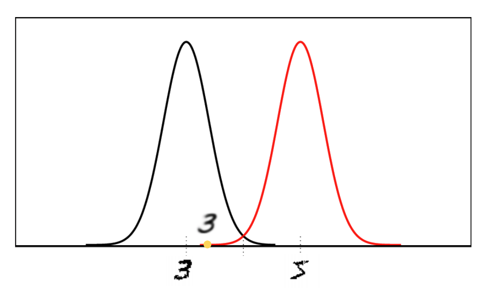
We can understand this in the other view. When a latent variable is sampled from the low-probability region of a latent distribution, it would inevitably lead to a bad reconstruction.

For the example in Fig 2, if we unfortunately sample a latent variable from the distribution of digit “5” (red) in the orange point, it turns out that this latent variable actually lies in the high probability region of the latent distribution generated by digit “3” (black) and it’s highly possible that we get a final reconstruction more similar to “3” rather than “5”. To make the posterior distribution close to the normal distribution, the regularizer will penalize this sample heavily by decreasing the variance, leading to a small spearout of the latent distribution. This drawback motivates the work of Importance Weight Autoencoders (IWAE) to introduce the importance weights into VAE, where a sampled latent variable which is far away from the mean will get assigned a lower weight during updates since it is known to give a bad reconstruction with high probability.

Importance Weighted Autoencoders

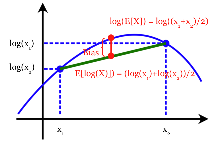
Another way to derivate ELBO is through the Jensen’s Inequality. Since $\log{(\cdot)}$ is a concave function, we have

$$\begin{align}\log{p_{\theta}(x)}&=\log{\mathbb{E}_{q_{\phi}(z|x)}[\frac{p_{\theta}(x,z)}{q_{\phi}(z|x)}]}\\ &\geq\mathbb{E}_{q_{\phi}(z|x)}[\log{\frac{p_{\theta}(x,z)}{q_{\phi}(z|x)}}]\\ &=\mathcal{L}_{\theta,\phi}(x).\end{align}$$

A simple example is shown in Fig 3. Consider a random variable $X$ taking value from $\{x_1, x_2\}$, and we want to estimate $\log{\mathbb{E}[X]}$. If we use $\mathbb{E}[\log{X}]$ to estimate it, then the estimation will converge at $\frac{\log{x_1}+\log{x_2}}{2}$, and the bias term cannot be eliminated by simply increasing the sampling times.

Fig 3. Bias in log expectation estimation

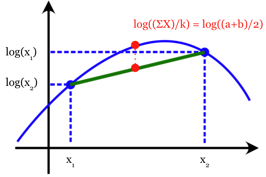
If we instead use $\mathbb{E}[\frac{1}{k}\sum_{i=1}^k{\log{X_i}}]$ for estimation, when we gradually increase the sampling times $k$, the bias will become smaller. And when $k\rightarrow+\infty$, the term inside the expectation actually becomes a constant which is exactly $\log{\mathbb{E}[X]}$, as shown in Fig 4.

Fig 4. Reducing the bias in the log expectation

If we apply this property on ELBO estimation, let $w_i=\frac{p_{\theta}(x,z_i)}{q_{\phi}(z_i|x)}$ and $\mathcal{L}_k=\mathbb{E}_{q_{\phi}(z|x)}[\log{\frac{1}{k}\sum_{i=1}^kw_i}]$, we actually have the theorem

$$\begin{align} \log{p_{\theta}(x)}\geq\mathcal{L}_{k+1}\geq\mathcal{L}_k. \end{align}$$

And $\mathcal{L}_k$ will converge to $\log{p_{\theta}(x)}$ when $\frac{p_{\theta}(x,z)}{q_{\phi}(z|x)}$ is bounded.

Equipped with this theorem, IWAE simply replace sthe objective in VAE with $\mathcal{L}_k$, where $k>1$. This gives a tighter lower bound compared with ELBO. And when $k=1$, IWAE is reduced to VAE.

In the backward pass, the gradient of $\mathcal{L}_k$ can be written as

$$\begin{align}\nabla_{\theta,\phi}\mathcal{L}_k&=\mathbb{E}_{q_{\phi}(z|x)}[\nabla_{\theta,\phi}\log{\frac{1}{k}\sum_{i=1}^kw_i}]\\ &=\mathbb{E}_{q_{\phi}(z|x)}[\sum_{i=1}^k\tilde{w_i}\log{\nabla_{\theta,\phi}w_i}], \end{align}$$

where $\tilde{w_j}=\frac{w_j}{\sum_{i=1}^kw_i}$ is the normalized importance weights, which makes the model name “Importance Weighted” Autoencoders. In VAE, $\tilde{w_j}$ takes the value $1$.

The meaning of the importance weights could be interpreted as this: if a latent sample itself has low probability in the latent distribution, then it should get assigned a lower weight in the gradient update since it’s known to cause a bad reconstruction with high probability. Introducing importance weights can effectively lower the risk shown in Fig 2.

Variants of IWAE

To make a straightforward comparison with ELBO in VAE, we fix the sampling times for both VAE and IWAE as $k$. The ELBO for IWAE and VAE become

$$\begin{align} \text{ELBO}_{\text{IWAE}}&=\log{\frac{1}{k}\sum_{i=1}^kw_i}\\ \text{ELBO}_{\text{VAE}}&=\frac{1}{k}\sum_{i=1}^k\log{w_i}. \end{align}$$

The main difference here is the position of the average operation, either insider or outside $\log{(\cdot)}$. IWAE regards the sampling outside $\log{(\cdot)}$ as the variance reduction, and it’s shown that IWAE actually doesn’t suffer from the large variance, so IWAE puts all sampling inside $\log{(\cdot)}$ to reduce the bias as much as possible.

However, a follow-up work [3] of IWAE theoretically proves that the sampling outside $\log{(\cdot)}$ is crucial to the training of the encoder. A tighter bound used by IWAE helps the generative network (decoder) but hurts the inference network (encoder).

Based on this discovery, three new models combining $\text{ELBO}_{\text{IWAE}}$ and $\text{ELBO}_{\text{VAE}}$ are proposed. For the following text, we fix the total sampling times to be $MK$, where $M$ is the sampling times outside $\log{(\cdot)}$ and $K$ is the sampling times inside $\log{(\cdot)}$.

• MIWAE. MIWAE simply uses an ELBO objective with both $M>1$ and $K>1$, i.e.,
  $$\begin{align} \text{ELBO}_{\text{MIWAE}}=\frac{1}{M}\sum_{m=1}^M\log{\frac{1}{K}\sum_{k=1}^Kw_{m,k}}. \end{align}$$
• CIWAE. CIWAE uses a convex combination of two ELBOs, i.e.,
  $$\begin{align} \text{ELBO}_{\text{CIWAE}}=\beta\text{ELBO}_{\text{VAE}}+(1-\beta)\text{ELBO}_{\text{IWAE}}. \end{align}$$
• PIWAE. PIWAE uses different objectives for the inference network and generative network. For the generative network, it keeps the objective of IWAE, $\text{ELBO}_{\text{IWAE}}$. While for the inference network, it switches to the objective $\text{ELBO}_{\text{MIWAE}}$.

Experimental Results

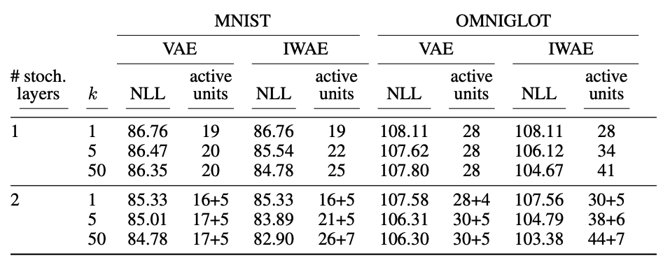
The experimental results demonstrate the advantage of IWAE against VAE as Table 1 shows. IWAE achieves lower negative log-likelihood (NLL) and more active units (active units captures data infomation) on all datasets and model architectures. And as $k$ increases, the performance is better since the lower bound is tighter.

Table 1. IWAE results

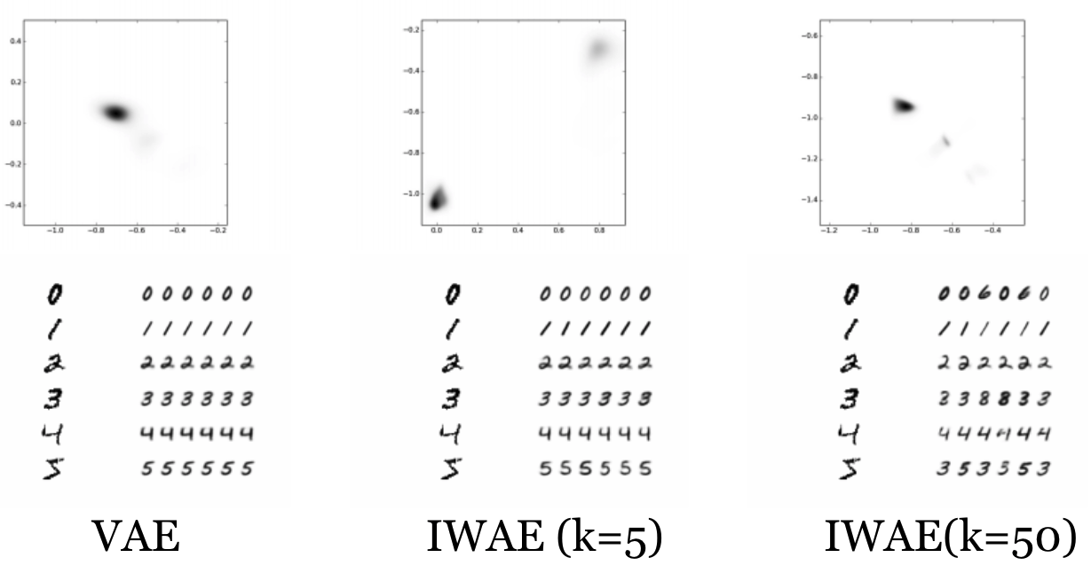
For the qualitative analysis in Fig 5, it’s worth noting that for IWAE, it has a larger spredout of the latent distribution and sometimes different output digits, e.g., “6” for “0”. This demonstrates the relaxation of the heavy panelization on the outliers, contrary to the example in Fig 2.

Fig 5. Ouput samples from VAE and IWAE

In a grid search of different combinations of $(M,K)$ with $MK$ fixed as $64$, we can see neither $M=1$ or $K=1$ makes the optimal solution in Fig 6. In other words, the ELBO objective should consider both the sampling inside and outside $\log{(\cdot)}$, which are beneficial to the generative network and inference network respectively.

Fig 6. Ouput samples from VAE and IWAE

Conclusion

IWAE uses a simple technique, moving the average operation inside $\log{(\cdot)}$, to achieve a tighter lower bound. The importance weights relaxes the heavy penalization on the posterior samples which fail to explain the observation. Although IWAE effectively reduces the bias, it’s shown that the sampling inside $\log{(\cdot)}$ is only beneficial to the generative network, but hurts the inference network. Therefore, to combine the ELBO in VAE and IWAE, the IWAE variants, MIWAE, CIWAE and PIWAE are proposed. The final results demonstrate that the optimal objective needs the sampling inside and outside $\log{(\cdot)}$ to be both greater than one. These works takes a deep look into the ELBO objective in VAE and reveal its role in the learning process.

References

• [1] 2014 (ICLR): D. Kingma, M. Welling, Auto-Encoding Variational Bayes, ICLR, 2014.
• [2] 2016 (ICLR): Y. Burda, R. Grosse, R. Salakhutdinov. Importance Weighted Autoencoders. ICLR, 2016.
• [3] 2018 (ICML): T. Rainforth, A. Kosiorek, T. Le, C. Maddison, M. Igl, F. Wood, Y. Teh, Tighter Variational Bounds are Not Necessarily Better. ICML, 2018.