VAE2 Improved Inference, Representation

Ladder VAE

Introduction

Ladder VAE was introduced in 2016, just after the introduction of VAE. And the purpose of LVAE was to explore how we can change the variational inference part of VAE to improve the performance without changing the generative model. It recursively corrects the generative distribution by a data dependent approximate likelihood.

Review of VAE

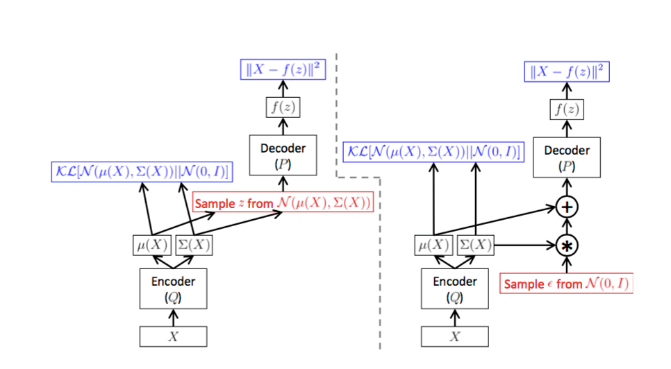
VAE models are made by two parts: the inference part and the generative part. The inference part takes an observation X and learns a latent representation of the input X and outputs a posterior distribution, usually Gaussian. Variational here means that the posterior learnt is approximate since the actual posterior distribution is not observable. The generative part takes a sample z from the latent posterior distribution learnt by the inference part and then learns to reconstruct the original observation X corresponding to this latent representation. And this is called the encoder-decoder structure.

The Problem

VAE model has some nice properties, for example, VAE is highly expressive, which means that they can learn a pretty good latent representation and generate vivid samples. VAE is also flexible and computationally efficient in most cases.

But due to the hierarchies of conditional stochastic variables, it is difficult to optimize when the model gets deep.

The paper found that purely bottom-up inference normally used in VAEs and gradient ascent optimization are only to a limited degree able to utilize the two layers of stochastic latent variables,
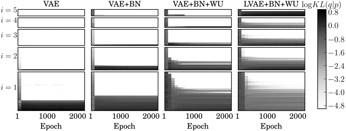
e.g. If you train a vanilla VAE with 5 layers, you will see that only the first two layers learn something, and the other layers are all inactive.

Thus, previous work on VAEs have been restricted to shallow models with one or two layers of stochastic latent variables. The performance of such models is constrained by the restrictive mean field approximation to the intractable posterior distribution. There are evidences suggesting that a more complex model often means better performance, and the research conducted here is following that direction which eventually becomes a cornerstone for further researches on deep VAE models like $\beta$-VAE framework.

Main Contribution

The paper’s main contribution is on:

1. Investigated into the inability of oridnary VAE to train deep hierachical stochastic layers.

2. Proposed Ladder VAE architecture to support deep hierarchical encoder, proposed LVAE which changes a bit of the inference model.

3. Verified the importance of BatchNormalization(BN) and Warm-Up(WU) to VAE.
   Made comparisons on VAE models with/without BN and WU to see the influence of BN and WU on the models. And turns out these techniques are essential for good performance.

Model Architecture

Ladder VAE model combines the approximate Gaussian likelihood with the generative model. According to the authors, ordinary VAE has no information sharing between encoder and decoder and this might be a bottleneck for learning a consistent posterior distribution. Thus, the proposed Ladder VAE model adds information sharing between the inference part and generative part. As the illustration below, Ladder VAE model (right) added deterministic upward nodes. Then during the stochastic downward pass, parameters are shared between the inference part and the generative part, while ordinary VAE model (left) has no information sharing between the two latent models.

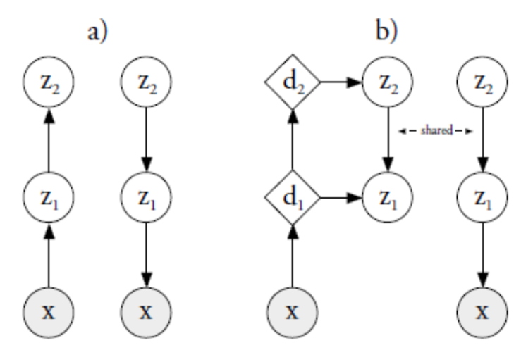
To perform a forward pass for the encoder, there would first be a deterministic upward pass computes the approximate likelihood contribution, followed by a stochastic downward pass recursively computing both the approximate posterior and generative distributions.

The approximate posterior distribution can be viewed as merging information from a bottom up computed approximate likelihood with top-down prior information from the generative distribution,

The sharing of information (and parameters) with the generative model gives the inference model knowledge of the current state of the generative model in each layer and the top down-pass recursively corrects the generative distribution with the data dependent approximate log-likelihood using a simple precision-weighted addition.

Objective Function

Ladder VAE model also uses Evidence Lower Bound (ELBO) as objective function:
$\log p(x)\ge E_{q_\phi(Z|X)}[\log \frac{p_\theta(x,z)}{q_\phi(Z|X)}]=L(\theta,\phi;x)$
$=-\beta KL(q_\phi(z|x)||p_\theta(z))+E_{q_\phi(Z|X)}(\log p_\theta(x|z))$
where $KL$ here is the KL-diveregence

Notice that there is an extra $\beta$ term in front of the KL-divergence term. This is what so called Warm-Up, which increases from 0 to 1 gradually during training time. The purpose of such “slow start” is to prevent high order layers of Ladder VAE from overfitting in early stage of training.By gradually introduce the KL-divergence, which is the variational regularization term used for regularizing the approximate posterior for each unit towards its own prior, the modified ELBO would start with reconstruction error term only and give high order layers sometime to learn useful information instead of ignoring them all before they can learn anything useful.

Generative Architecture

The generative part is the same for both VAE and Ladder VAE
$p_\theta(z)=p_\theta(z_L)\prod_{i=1}^{L-1}p_\theta(z_i|z_{i+1})$
$p_\theta(z_i|z_{i+1})=N(z_i|\mu_{p,i}(z_{i+1}),\sigma^2_{i+1}(z_{i+1}))$
$p_\theta(z_L)=N(z_L|0,I)$
$p_\theta(x|z_1)=N(x|\mu_{p,0}(z_1),\sigma^2_{p,0}(z_1))$

Inference Architecture

For VAE model
KaTeX parse error: Unexpected character: '�' at position 1: �̲�(𝑦)=MLP(𝑦)
KaTeX parse error: Unexpected character: '�' at position 1: �̲�(𝑦)=Linear(𝑑…
KaTeX parse error: Unexpected character: '�' at position 11: \sigma^2 (�̲�)=Softplus(Lin…

$q_\phi(z|x)=q_\phi(z_1|x)\prod_{i=2}^Lq_\phi(z_i|z_{i-1})$
$q_\phi(z_1|x)=N(z_1|\mu_{q,1}(x),\sigma^2_{q,1}(x))$
$q_\phi(z_i|z_{i-1})=N(z_i|\mu_{q,i}(z_{i-1}),\sigma^2_{q,i}(z_{i-1})),i=2\ldots L$

For Ladder VAE model
$d_n=MLP(d_{n-1}),d_0=x$
$\hat\mu_{q,i}=Linear(d_i),i=1\ldots L$
$\hat\sigma^2_{q,i}=Softplus(Linear(d_i)),i=1\ldots L$
$\sigma_{q,i}=\frac{1}{\hat \sigma^{-2}_{q,i}+\sigma^{-2}_{p,i}}$
$\mu_{q,i}=\frac{\hat\mu_{q,i}\hat\sigma^{-2}_{q,i}+\mu_{p,i}\sigma^{-2}_{p,i}}{\hat \sigma^{-2}_{q,i}+\sigma^{-2}_{p,i}}$
$\sigma_{q,L}=\hat\sigma_{q,L},\mu_{q,L}=\hat\mu_{q,L}$
$q_\phi(Z_i|\cdot)=N(z_i|\mu_{q,i},\sigma^2_{q,i})$

Experimental Results

The paper conducted experiments on both MNIST dataset and OMNIGLOT dataset and here I show the main results.

Results on MNIST dataset

Results on OMNIGLOT dataset

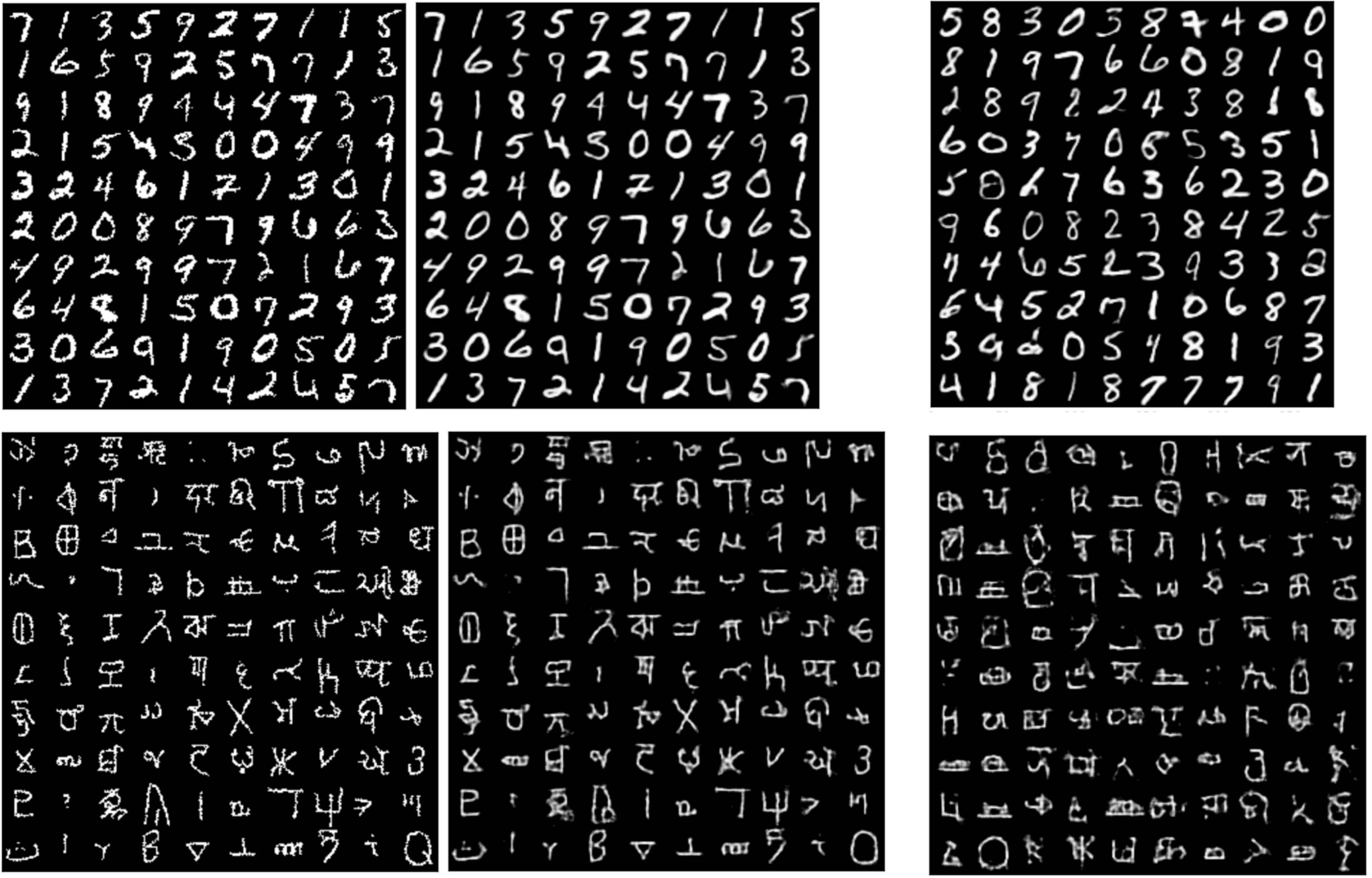
Samples from both datasets. The left part of the image is a illustration of sample reconstruction for Ladder VAE, where the left most image is ground truth and the middle image is the reconstructed image. On the right, the top part are samples drawn from MNIST dataset and the bottom part are samples drawn from OMNIGLOT dataset.

They also recorded the log-likelihood for each layer in throughout the training to compare the number of active units in each layer at each timestep. And from the plot one can see that ordinary VAE can’t train layers above 2 while Ladder VAE model and VAE model+BN+WU have significantly more active units in high order layers.

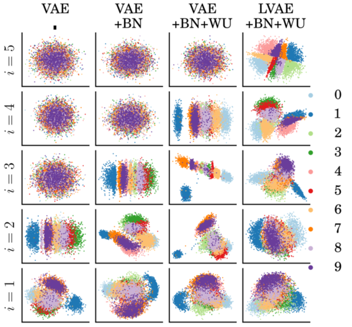
Layer-wise PCA analysis has shown that Ladder VAE model is able to learn much more useful information in high order layers than ordinary VAE model.

Vector-Quantized VAE

Vector Quantized VAE (VQ-VAE) aims to train an expressive VAE model using discrete latent space.

Motivation and Approach

VQ-VAE borrowed ideas from Vector Quantization in compression algorithms, which is a classical quantization technique from signal processing that allows the modeling of probability density functions by the distribution of prototype vectors. It works by dividing a large set of points (vectors) into groups having approximately the same number of points closest to them. Each group is represented by its centroid point, as in k-means and some other clustering algorithms.

Thus, the posterior now becomes:

where $z_e$ is the ordinary continuous latent code given by encoder, $e_j$ is a discrete latent embedding. So that VQ-VAE is essentially adding an extra quantization layer between ordinary VAE encoder and decoder.

Main Contribution

The main contribution of VQ-VAE is they adapted a discrete latent space (their encoder generates discrete latent codes), so that their model achieves extrodinary dimension reduction while maintaining a good performance. By using discrete latent codes, VQ-VAE has a smaller variance and they also managed to circumvent the problem of posterior collapse which happens when decoder ignores samples from posterior when it’s too weak or too noisy.

Objective

The objective function of VQ-VAE is made up by three parts:
$L=\log p(x|z_q(x))+||sg[z_e(x)]-e||^2_2+\beta||z_e(x)-sg[e]||^2_2$
where $sg$ stands for stop gradient operator which is defined as identity during forward pass and has zero partial derivative, thus constraining its operand to be a non-updated constant.

Here, the first term is reconstruction Loss which optimizes encoder-decoder. The second term is VQ Objective which Learns the latent embedding. And the last term is commitment loss, used to
make sure the encoder commits to an embedding and its output does not grow.
Since the volume of the embedding space is dimensionless, it can grow arbitrarily if the embeddings $e_j$ do not train as fast as the encoder parameters

Experiments

The paper conducted experiments on image, audio, and video stream and here I show some results for images.

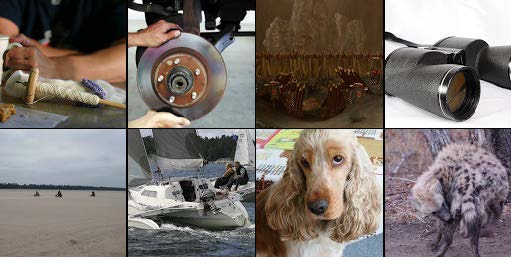
Below is an example of image reconstruction, the top is ground truth and the bottom is reconstructed image.

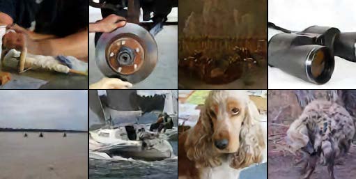
Below are exmaples of sampled images from VQ-VAE.

Reference

• Casper Kaae Sønderby, Tapani Raiko, Lars Maaløe, Søren Kaae Sønderby, and Ole Winther. Ladder Variational Autoencoders. Neural Information Processing Systems, 2016