VAE3 Deep Hierarchical

Introduction

This blogpost talks about deep hierarchical VAEs - why do we need deep (instead of shallow) hierarchy, what are the main challenges, and how do to design them.

It is commonly known that VAE variants generates much less realistic images than GANs. One major hypothesis is that the latent space sturcure is too limited: there is no hierarchy and we try to fit a simple prior (e.g. a standard Gaussian) to it. When we want to increase its capacity while keeping the divergence loss tractable, the idea of hierarchy naturally comes to mind.

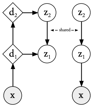
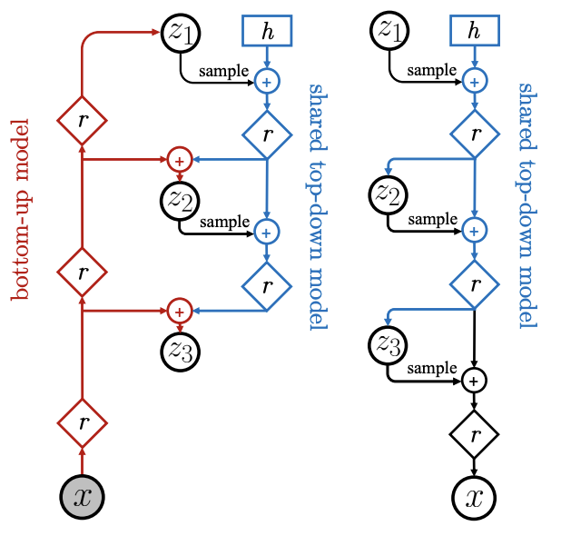
Ladder VAE (LVAE) is an early example of hierarchical VAE. In addition to dividing the latent space into multiple layers, it also enables bidirectional (bottom up and top-down) flow of information from layer to layer. The models we will discuss below are based heavily on its design.

Architecture of very deep hierarchical VAE.

The latter structure alone doesn’t bridge the gap bbetween GANs and VAEs, but we will see below that models based on its design will finally reach a performance comparable to SOTA generative models.

NVAE

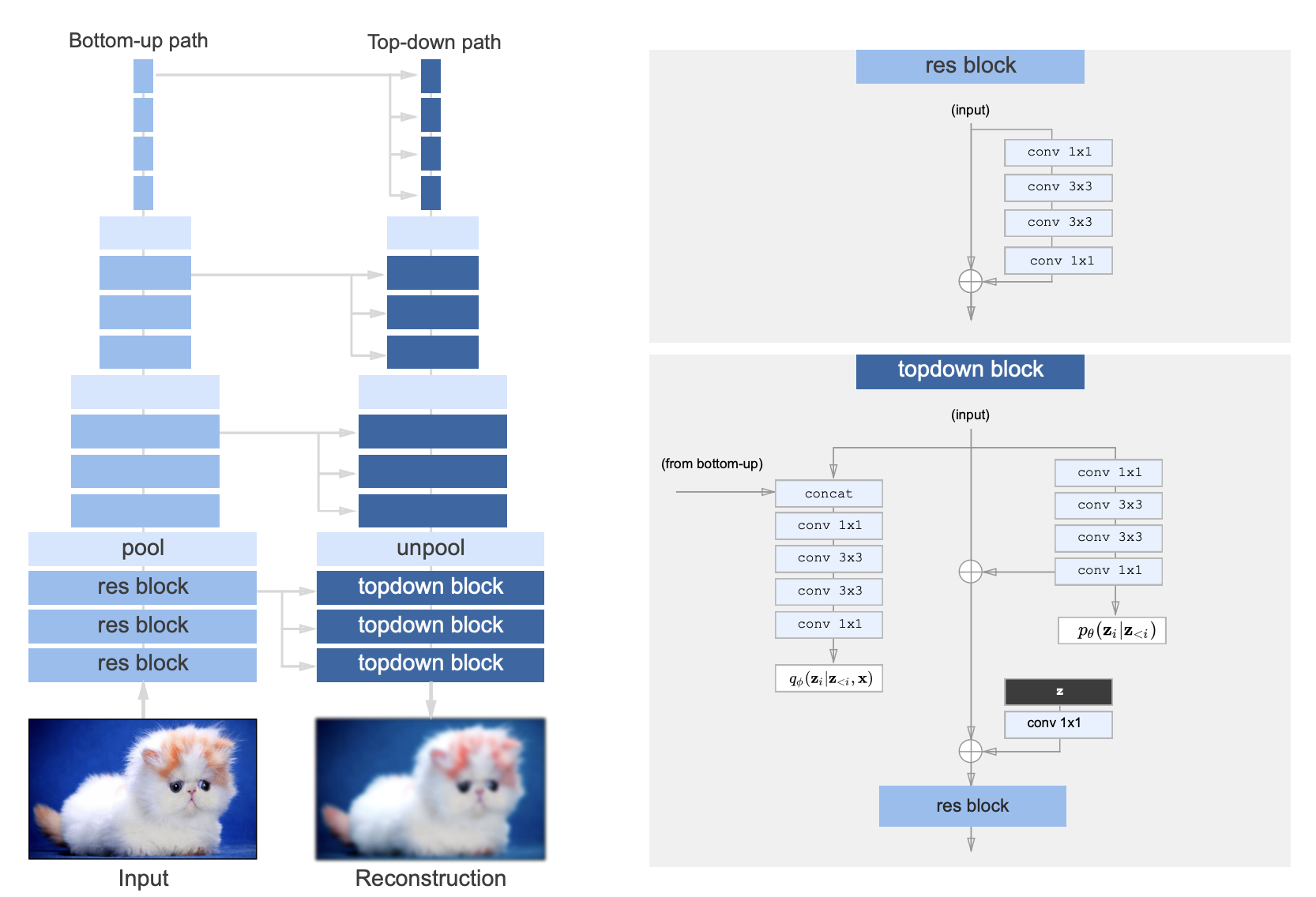
Nouveau VAE (NVAE) focuses on improving performance through architecture refinement. The hierarchical architecture is based on LVAE, but with difference scale per layer of latent variables.

VAE model

There are four main improvements:

Residual Cells in Encoder and Decoder

Adding residual connection to VAE is easy, but to realize long-range correlation in data is tricky. One straightforward way is to increase the kernel size of convolution layers in the decoder, but then we face the problem of large parameter sizes. To solve this problem, NVAE uses depthwise separable convolution from MobileNetV2 ¹.

Other components of the residual cells include:

batch normalization (BN) to replace weight normalization (WN)
Swish activation $f(u) = \frac{u}{1 + \exp(-u)}$ to replace ELU
final Squeeze and Excitation (SE）layer inspired by SENet ²

Residual Normal Distribution

Deep hierarchical VAE suffers from the problem of instable KL divergence. Unlike the vanilla VAE which assumes a standard Gaussian prior $p(z) = \mathcal{N}(0, I)$ , in each layer of LVAE both the posterior $q(z_l \mid x, z_{<l})$ and the prior $p(z_l \mid z_{<l})$ are generated from previous layers, making it very challenging to match the two distributions.

This problem can be solved via reparametrizing the posterior using residual distribution $\Delta\mu$ and $\Delta\sigma$ . That is, $q(z_l \mid z_{<l}, x) = \mathcal{N}(\mu(z_{<l}) + \Delta\mu(z_{<l}, x), \sigma(z_{<l})\cdot\Delta\sigma(z_{<l},x))$ .

Under this parametrization, when the prior $p(z_l \mid z_{<l})$ changes, the posterior $q(z_l \mid z_{<l}, x)$ moves accordingly.

Another way to interpret this change is to derive the expression for KL divergence: $D_{KL}(q(z \mid x), p(z)) = \frac{1}{2}(\frac{\Delta\mu^2}{\sigma^2} + \Delta\sigma^2 - \log\Delta\sigma^2 - 1)$ . When $\sigma^2$ is bounded from below, the term is mainly dependent on the encoder’s output, and therefore it’s easier to minimize KL divergence compared to the standard parametrization, where KLD is dependent on the outputs of both the encoder and the decoder.

Spectral Regularization (SR)

To ensure that the encoder doesn’t produce drastically different latent codes when the input slightly changes, it would be nice if it is made Lipschitz. To achieve this end $\mathcal{L}_{SR} = \lambda\sum_i s^{(i)}$ is added as a regularization loss, where $s^{(i)}$ is the largest singular value of the $i$ -th convolution layer. Spectral regularization ³ is shown to minimize the Lipschitz constant for each layer.

Normalization Flows (NFs) for Generating Posterior

Finally, n order to further increase expressivity of the posterior distributions, a few IAF ⁴ layers are appended to the encoder.

Very Deep Hierarchical VAE

In the other paper ⁵, the authors claim that deep hierarchical VAEs generalize autoregressive models such as PixelRNN ⁶. The claims is proven in two theorems:

Proposition 1. N-layer VAEs generalize autoregressive models when N is the data dimension.
Proposition 2. N-layer VAEs are universal approximators of N-dimensional latent densities.

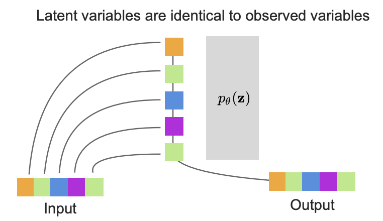
The first proposition can be intuitively understood through the following figure, while the second proposition trivially follows it if we admit that image domains usually have lower rank than their resolutions.

Hierarchical VAE that learns an autoregressive model.

Therefore, a hierarchical VAE that is deep enough should be able to reach the same level of sample quality as autoregressive models. The paper uses a slightly different variant of LVAE (but deeper), but also with multi-scale layers and residual blocks.

Architecture of very deep hierarchical VAE.

Experiments and Conclusion

The very deep hierarchical VAE paper provides a thorough investigation of different VAE as well as autoregressive models:

| Dataset | Model | Model Type | NLL |
| CIFAR-10 | Sparse Transformer | AR | 2.80 |
| CIFAR-10 | Flow++ | Flow | $\le$ 3.08 |
| CIFAR-10 | NVAE | VAE | $\le$ 2.91 |
| CIFAR-10 | Very Deep VAE | VAE | $\le$ 2.87 |
| ImageNet-32 | Image Transformer | AR | 3.77 |
| ImageNet-32 | Flow++ | Flow | $\le$ 3.86 |
| ImageNet-32 | NVAE | VAE | $\le$ 3.92 |
| ImageNet-32 | Very Deep VAE | VAE | $\le$ 3.80 |
| ImageNet-64 | Sparse Transformer | AR | 3.44 |
| ImageNet-64 | Flow++ | Flow | $\le$ 3.69 |
| ImageNet-64 | Very Deep VAE | VAE | $\le$ 3.52 |
| FFHQ-256 | NVAE | VAE | $\le$ 0.68 |
| FFHQ-256 | Very Deep VAE | VAE | $\le$ 0.61 |
| FFHQ-1024 | Very Deep VAE | VAE | $\le$ 2.42 |

In conclusion, Very Deep VAE is able to reach the same level of sample quality as SOTA autoregressive and NF methods. Also it can be trained on high-resolution datasets, which no previous VAE has attempted.

Although it seems trivial to expand LVAE architecture to a larger scale, successfully doing so actually requires paying attention to various details. The proof that VAEs have the capacity to generate images as good as autoregressive models or NFs do is also meaningful and inspiring for future research.